"The end-to-end policy learned something. What it learned is between the gradients and the weights, and neither will tell you."
A Diagnostic Engineer With No Intermediate Representations
The ideas introduced here are extended in section 3.4, which shows how learned policies are embedded inside hybrid and hierarchical architectures. The behavior-cloning formulation used in the worked example is treated in full in section 21.2, and the action-chunking and diffusion variants that address compounding errors are developed in section 22.2. Vision-language-action models, including RT-2 cited below, are examined as a class in section 34.2.
A robot hand picks up a mug by reading raw pixels and writing motor torques, with no hand-coded depth estimator, no explicit grasp planner, no rule saying "align fingers before closing." The entire skill lives in a single neural network trained end-to-end on demonstrations. This is not a thought experiment: systems like RT-2 and ACT do exactly this today, and they generalize to objects they have never touched. The reason this matters now is that the alternative, stacking separately tuned modules, accumulates error at every handoff and breaks the moment one module drifts. Here you will understand why a monolithic learned policy can outperform that pipeline, what the training objective actually optimizes, and where the architecture bites back when things go wrong.
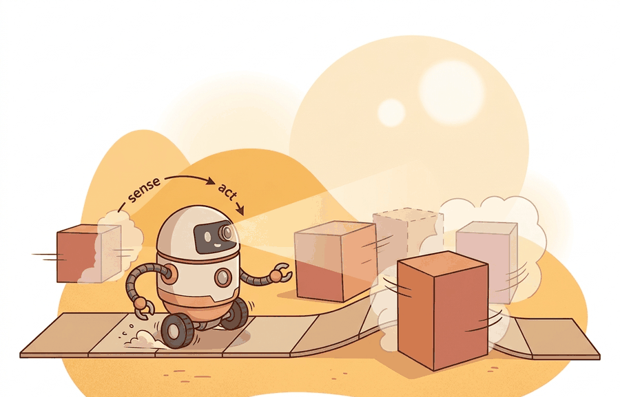
The end-to-end policy collapses evidence, decision, and consequence into one learned map, and the dashed feedback arrow shows why this matters: because each action reshapes the next observation, there are no intermediate modules to inspect when the loop drifts, so the first diagnostic becomes a data-coverage audit rather than a module trace. This is the same diagram introduced as Figure 1.3.
Strip out the depth estimator, the grasp planner, and every "if-then" rule a roboticist would normally write, replace the whole stack with one neural network from pixels to torques, and you get a policy that grasps mugs it has never seen, yet offers nothing to inspect the moment it fails. That is the bargain of the end-to-end learned policy pipeline, and this section makes it usable. Figure 3.3A shows the shape of the idea: raw camera pixels enter a single neural network that directly outputs motor torques, with learned layers replacing every explicit intermediate module. Figure 3.3 reframes the same architecture as a closed-loop evidence, decision, consequence pattern, where each action changes the next observation. The section defines the object of study, connects it to the agent loop, and tests it with a compact implementation.
The key question is practical: what must the agent know, what can it observe, what action is available, and what evidence shows that the action worked under the stated conditions?
The word "pipeline" in this section's title does not mean a chain of separately-coded modules; it means the sequence of stages a builder still has to run even when a single network makes the moment-to-moment decision: collect demonstrations, normalize actions, train the network, and audit coverage before deployment. Each of those stages appears later in this section (the Algorithm callout below walks through exactly these steps), so "end-to-end" describes the runtime decision, while "pipeline" describes the surrounding workflow that produces and checks that decision.
A representation earns its place when it changes the measurable action interface. In end-to-end learned policy pipeline, the reader should keep asking which decision becomes easier, safer, or more reliable.
Theory
The practical design rule is to make the interface inspectable before optimization begins: inputs, outputs, units, latency, bounds, and failure labels should all be visible in the saved artifact.
An end-to-end policy is motivated by the handoff problem in modular stacks: if perception produces exactly the wrong abstraction, the planner never sees the information it needed. Instead of committing to intermediate symbols, the policy learns a direct map from observations and goals to actions:
$$a_t = \pi_\theta(o_{\le t}, g), \qquad \theta^\star = \arg\min_\theta \sum_{(o,g,a^\star)} \ell(\pi_\theta(o,g), a^\star).$$
The policy replaces every intermediate symbol with one learned map from observation and goal to action, trading module-level transparency for representation freedom.
The loss \(\ell\) is often a regression loss for continuous actions, a cross-entropy loss for discrete action tokens, or a diffusion-style denoising loss for action chunks. The benefit is representation freedom: the model can keep visual, temporal, and language cues that a hand-written state estimator might discard. The cost is diagnostic opacity without intermediate symbols. A policy that cannot be inspected module by module is typically not less fragile; it is fragile in a way that is harder to see. When the policy fails, the builder must probe data coverage, action scaling, temporal context, embodiment mismatch, and distribution shift rather than open a single broken module. The coverage stakes are concrete. Behavior-cloning evaluations through 2024 (ACT, Zhao et al. 2023; OpenVLA, Kim et al. 2024) show that a policy trained on roughly 50 in-distribution demonstrations reaches 80-90% task success within that distribution. The same policy drops below 20% on observations roughly 2x outside the training range. In these reported evaluations, that gap tracks data coverage far more closely than model capacity (though the two are not fully separable, since a larger model can also partially compensate for sparse coverage). Adding around 150 diverse demonstrations recovers performance above 70% with no architecture change in those same evaluations. In other words, in this evidence, the difference between a robot that works and one that fails is closer to 150 extra teleoperated episodes than to a bigger network.
Algorithm: Behavior-Cloning Policy Training and Coverage Audit
Input: demonstration dataset \(\mathcal{D} = \{(o_i, g_i, a_i^\star)\}_{i=1}^{N}\), learning rate \(\alpha\), policy network \(\pi_\theta\) with parameters \(\theta\), query observation \(o_q\) at deployment time
Output: trained parameters \(\theta^\star\), predicted action \(\hat{a} = \pi_{\theta^\star}(o_q, g)\), coverage score \(c(o_q)\)
- Compute per-dimension mean \(\mu_a\) and standard deviation \(\sigma_a\) over all \(a_i^\star \in \mathcal{D}\); normalize actions as \(\tilde{a}_i = (a_i^\star - \mu_a) / \sigma_a\). Store \((\mu_a, \sigma_a)\) alongside the checkpoint.
- Initialize \(\theta\) (e.g., random or from a pretrained backbone). Set iteration counter \(t \leftarrow 0\).
- Sample a mini-batch \(\mathcal{B} \subset \mathcal{D}\). Compute the imitation loss: \(\mathcal{L}(\theta) = \frac{1}{|\mathcal{B}|} \sum_{(o,g,\tilde{a}^\star) \in \mathcal{B}} \ell\!\left(\pi_\theta(o, g),\, \tilde{a}^\star\right)\).
- Compute gradient \(\nabla_\theta \mathcal{L}(\theta)\) via backpropagation.
- Update parameters: \(\theta \leftarrow \theta - \alpha\, \nabla_\theta \mathcal{L}(\theta)\). Increment \(t\).
- Repeat steps 3-5 until convergence or the iteration budget is exhausted. Record \(\theta^\star \leftarrow \theta\).
- At deployment, obtain query \(o_q\). Predict raw action \(\hat{a}_{\text{raw}} = \pi_{\theta^\star}(o_q, g)\); recover physical units: \(\hat{a} = \sigma_a \cdot \hat{a}_{\text{raw}} + \mu_a\).
- Compute coverage score: \(c(o_q) = \frac{1}{k}\sum_{j=1}^{k} \|o_q - o_{(j)}\|_2\), where \(o_{(1)}, \ldots, o_{(k)}\) are the \(k\) nearest training observations to \(o_q\).
- If \(c(o_q)\) exceeds a threshold \(\tau\), flag the query as out-of-distribution before accepting \(\hat{a}\).
- Log \((o_q, g, \hat{a}, c(o_q))\) as a structured failure record if the rollout does not succeed, to distinguish coverage failures from representation-alignment failures.
Before training, normalize every action dimension to zero mean and unit variance using statistics computed over the full demonstration dataset, then store those statistics alongside the model checkpoint. LeRobot's normalize_action utility and ACT's reference implementation both do this automatically, but custom pipelines routinely skip it. A policy trained on raw joint-angle targets (which span different ranges per joint) will saturate the output head on joints with large variance and produce near-zero commands on joints with small variance, causing the robot to appear "frozen" on some axes while overcorrecting on others. The fix at inference time is to apply the inverse transform using the saved mean and std before sending commands to the controller.
The algorithm above is a template; real published systems fill in its steps with different network sizes and datasets, which is why the numbers below vary so much between systems. Consider a specific case. RT-2 (Brohan et al., 2023) fine-tunes a 55-billion-parameter vision-language model to output robot joint commands as text tokens. By transferring web-scale visual semantics, it reaches 62% success on novel objects and categories absent from the robot training data. Action Chunking with Transformers (ACT, Zhao et al., 2023) takes a different point on the design curve. A smaller 80-million-parameter transformer trains on 50 human demonstrations per task and hits 80-90% success on precise bimanual manipulation. It predicts 100-millisecond action chunks (short bursts of future actions produced in one forward pass, defined in detail two paragraphs below) that smooth out compounding errors. OpenVLA (Kim et al., 2024) shows the same vision-language-action (VLA) recipe scales to open weights at 7 billion parameters, matching RT-2 manipulation success at roughly one-tenth the inference cost. These three systems span the specificity-versus-cost tradeoff the formula above leaves open. The observation space and action tokenization differ, but the direct \(o \to a\) mapping stays constant across all three.
Checkpoint
So far: an end-to-end policy learns a direct observation-to-action map trained with a regression, cross-entropy, or diffusion-style loss; that map trades away inspectable modules for representation freedom; and three real systems (RT-2, ACT, OpenVLA) show this same \(o \to a\) recipe working at very different model sizes and costs. The next paragraphs explain the one design choice, action chunking, that most improves stability on physical hardware.
ACT earned its strong numbers above by predicting short action chunks rather than single steps. That single design choice accounts for much of the reported gain. The ACT paper's own ablations attribute the largest single improvement to chunking, though the final numbers also depend on the transformer architecture and the training data, so "most of the work" should be read as an ablation-supported estimate, not an exact decomposition. Action chunking matters in embodied AI because physical robots accumulate error over time: each single-step prediction adds noise, and the next prediction is conditioned on the now-corrupted state. On a real manipulator, this compounding causes the gripper to drift off the grasp axis within seconds. Predicting a short sequence of future actions in one forward pass breaks that feedback loop for the duration of the chunk, keeping the robot on a locally consistent trajectory without querying the policy at every timestep.
The mechanism works by changing the output head from a single action vector to a sequence of \(H\) consecutive actions. During training, the policy minimizes loss across all \(H\) steps jointly, so the network learns temporally consistent motion. At inference, the robot executes the chunk open-loop for \(H\) steps, then re-queries the policy. ACT uses a transformer encoder-decoder where the decoder autoregressively generates the chunk conditioned on a visual and proprioceptive token, where proprioception is the robot's sense of its own joint angles and gripper state, then executes all \(H\) outputs before the next observation is needed.
End-to-end policies outperform modular stacks when the right intermediate representation is unknown or contested: tasks that require fusing appearance, geometry, and language in ways no hand-written state estimator was designed to handle. They struggle when the training distribution is narrow relative to deployment variation, when the action horizon exceeds the model's temporal context window, or when safety requires a hard constraint the loss function cannot reliably enforce. A practical decision rule: choose end-to-end when you have broad, diverse demonstrations and no reliable symbolic state; choose a modular or hybrid stack when you have well-defined state variables, explicit safety limits, or a deployment environment that will shift faster than you can retrain.
The mechanism in End-to-end learned policy pipeline is the contract between representation and action. Name what enters the module, what leaves it, which assumptions make that transformation valid, and which log would reveal a bad handoff.
Worked Example
An end-to-end policy learns the map \(a = \pi_\theta(o, g)\) directly from demonstrations, with no hand-written state in between. The example fits a minimal behavior-cloning policy by least squares, then makes the section's central point: when it fails, the first diagnostic is not "open a module" but "audit data coverage." We do that with a nearest-neighbor check against the training set.
import numpy as np
rng = np.random.default_rng(0)

# Demonstrations: observation = [obj_x, obj_y], goal g = 1 (pick).
# Expert action = unit vector from a fixed gripper origin to the object.
N = 200
O = rng.uniform(-1, 1, size=(N, 2))          # objects in a seen region
A = O / np.linalg.norm(O, axis=1, keepdims=True)   # expert reach direction

# Behavior cloning by least squares: a = O @ W  (the whole "training run").
W, *_ = np.linalg.lstsq(O, A, rcond=None)

def policy(o):
    return o @ W

def coverage(o, k=5):                          # distance to k nearest demos
    d = np.linalg.norm(O - o, axis=1)
    return np.sort(d)[:k].mean()

for label, o in [("in-distribution", np.array([0.3, -0.4])),
                 ("far OOD",        np.array([3.0,  3.0]))]:
    a = policy(o)
    err = np.linalg.norm(a - o / np.linalg.norm(o))
    print(f"{label:16s} cover={coverage(o):.2f} action_err={err:.2f}")
lstsq weight solve and policy function), then runs the nearest-neighbor coverage audit that compares an in-distribution query against a far out-of-distribution query. The jump in coverage distance flags that the failed input is outside the training support before any architecture change is considered.Step-Through: nearest-neighbor coverage audit
Trace the coverage check with a tiny dataset of three demonstrations and no model at all, so the diagnostic logic is visible in raw numbers. Training observations: \(o_1=(0.0,\,0.0)\), \(o_2=(0.2,\,0.1)\), \(o_3=(-0.1,\,0.3)\). Use \(k=2\).
Query A (in-distribution), \(o_q=(0.1,\,0.1)\). Distances: to \(o_1\), \(\sqrt{0.1^2+0.1^2}=0.141\); to \(o_2\), \(\sqrt{0.1^2+0.0^2}=0.100\); to \(o_3\), \(\sqrt{0.2^2+0.2^2}=0.283\). The two nearest are \(0.100\) and \(0.141\), so \(c(o_q)=(0.100+0.141)/2=0.121\).
Query B (far OOD), \(o_q=(3.0,\,3.0)\). Distances: to \(o_1\), \(4.243\); to \(o_2\), \(4.072\); to \(o_3\), \(3.992\). The two nearest are \(3.992\) and \(4.072\), so \(c(o_q)=(3.992+4.072)/2=4.032\).
With threshold \(\tau=0.5\), Query A passes (\(0.121 < 0.5\)) and its action is accepted, while Query B is flagged out-of-distribution (\(4.032 > 0.5\)) and its action is rejected before execution. The coverage score jumped roughly 33x with no change to the policy weights, which is exactly the signal that the failure is a data-coverage gap, not a broken module.
Expected output: the in-distribution query has small coverage distance and bounded action error; the far out-of-distribution query has a large coverage distance and a much larger error (the linear policy cannot extrapolate the normalized reach direction it never saw). That contrast is the diagnosis: the policy is not "broken," it is being asked about a region it never saw. This is why the first isolation test for an end-to-end policy is a coverage audit, not a module trace, because the architecture deliberately removed the modules you would otherwise inspect.
Think of a chef who has spent years cooking by feel rather than following written recipes. The dish she produces can be extraordinary, but when it goes wrong, there is no recipe card to inspect, no intermediate step labeled "add salt here." You cannot open the chef's head and read off which stage failed; instead, you compare what ingredients were available that day against every past session where the dish succeeded. Diagnosing an end-to-end policy works the same way: the network has compressed every intermediate judgment into its weights, so the first diagnostic question is always "have we seen this situation before?" rather than "which module produced the wrong output?"
The hand-built fragment is a visibility tool. Production work should move to maintained stacks such as Hugging Face Transformers, open VLMs, OpenVLA, openpi, LeRobot, and tool-calling planners once the section has made the interface, logging contract, and failure recovery path explicit.
Practical Recipe
- Fix the observation contract before touching model architecture: specify camera resolution (e.g., 224x224 RGB at 10 Hz for ACT, 480x640 for RT-2), whether proprioception (joint angles, gripper state) is concatenated to the visual token, and the maximum acceptable sensor latency. A 20 ms timestamp mismatch between a wrist camera and joint encoders will corrupt the action-chunking temporal alignment and produce oscillating Franka Panda wrist commands even when the visual prediction is correct.
- Use a behavior-cloning baseline trained on 50 demonstrations as the first checkpoint, not a pretrained VLA. On a Franka tabletop pick-and-place task this baseline achieves 70-80% success and is fast enough to retrain overnight, making data-coverage failures visible before investing in fine-tuning a 7B-parameter OpenVLA checkpoint.
- Before adding more demonstrations, ask: what did the policy never see? A coverage audit on the failed rollouts typically reveals that the missing cases cluster in one corner of the workspace, one lighting condition, or one object orientation. Fixing that gap costs far less than doubling the total dataset size.
- Normalize every action dimension to zero mean and unit variance using per-joint statistics computed from your demonstration dataset, not from a generic prior. Store the normalization constants in the checkpoint. Franka joints span roughly -2.9 to 2.9 rad but finger joints span only 0 to 0.08 m; without per-joint normalization the output head saturates on shoulder joints and undercontrols the gripper, causing drops on pick tasks even when reach accuracy is good.
- Record failures with four fields: (a) nearest-neighbor coverage distance to the training set in observation space, (b) which joint or gripper axis shows the largest tracking error, (c) whether the episode terminated from a contact event or a timeout, and (d) whether the scene lighting or object pose was inside the distribution of training images. These four fields separate coverage failures, control failures, and sim-to-real appearance failures without opening the model weights.
- Before deploying on physical hardware, run one sim-to-real perturbation test in MuJoCo or Isaac Lab: apply a uniform random shift of plus or minus 15 cm to object position and record how success rate degrades. If success drops below 50% at 10 cm shift, the demonstration dataset covers too small a workspace volume; add scripted or teleoperated data from the perimeter of the target workspace rather than retraining from scratch.
A common assumption is that because an end-to-end policy replaces hand-coded rules with learned weights, it must generalize more broadly than a modular pipeline. This is wrong. Removing hand-coded modules does not add coverage; it only changes where the boundary lives. The policy is still a function fit to a finite dataset, and any observation outside that dataset's support typically produces extrapolated outputs whose quality is uncontrolled. In embodied AI the physical environment changes continuously, so a policy trained on 200 tabletop demonstrations in one lighting condition can, in practice, fail sharply when a lamp is moved or an object color shifts. The correct mental model is that an end-to-end policy trades transparent module boundaries for representation freedom, and that freedom comes with an obligation to audit data coverage, not an exemption from it.
The common mistake in End-to-end learned policy pipeline is to celebrate the component score before checking the closed-loop handoff. The failure usually appears at the boundary: stale state, wrong frame, delayed action, saturated actuator, or metric that ignores the real task cost.
When an ACT policy on a bimanual Franka setup logs only the final pick-success flag, a 78% number hides the fact that every success came from objects in the front-center 20 cm of the workspace, while the rear-corner placements timed out. Logging the per-step gripper pose, the LeRobot controller status, the termination reason (contact versus timeout), and the nearest-neighbor coverage distance turns that single flat number into a workspace-coverage map that shows exactly which teleoperated episodes are missing. The logs reveal whether the policy is solving the task or merely passing the easiest episodes.
Real-World Application: warehouse and home manipulation
Google DeepMind's RT-2 runs the full end-to-end recipe on a real mobile manipulator: raw camera frames and a language goal enter a single vision-language-action model that emits joint commands as text tokens, with no separate detector, grasp planner, or motion controller in between. The same monolithic-policy design underlies Physical Intelligence's pi0, which a startup fine-tunes in hours to fold laundry and bus tables on physical robots. In both systems the entire perception-to-torque skill lives in one network trained on demonstrations, exactly the \(o \to a\) map this section formalizes.
End-to-end learning removes the hand-coded middle. It also removes several convenient places to point when the robot gets creative.
1. Scalable robot foundation models via internet-scale data. The central 2024-2025 push is to scale behavior-cloning data far beyond single-lab teleoperation. Physical Intelligence's pi0 (Black et al., 2024) combines a pretrained vision-language backbone with a flow-matching action head (a continuous generative model that learns to transform noise into actions, closely related to the diffusion-style loss introduced above) and trains across 68 robot embodiments; it demonstrates that a single generalist checkpoint can be fine-tuned to new tasks in hours rather than weeks. Google DeepMind's GROOT and the Open X-Embodiment collaboration (2023-2024) extend this by pooling data across seven different robot platforms, showing that cross-embodiment pretraining reduces per-task sample requirements by roughly 3x on held-out manipulators.
2. Diffusion and flow-matching action heads replacing regression losses. Replacing the mean-squared-error (MSE) action head with a denoising diffusion or continuous normalizing flow objective sharpens multimodal action distributions and measurably improves dexterous task success. Chi et al. "Diffusion Policy" (2023, extended in robot deployments through 2025) and the Octo model (Team, 2024) both show that diffusion heads outperform deterministic regression heads by 10-20 percentage points on contact-rich tasks while adding only moderate inference-time compute. As of 2024-2025, this direction has become the default output head in most new open-source policy frameworks, including LeRobot's ACT-Diffusion variant and openpi.
3. Test-time adaptation and online fine-tuning without human resets. Deployed policies fail silently when environment conditions shift. The 2024-2025 frontier asks how a policy can detect its own uncertainty and self-correct without requiring a human to reset the scene. SERL (Luo et al., 2024, Berkeley RAIL Lab) demonstrates residual reinforcement learning (a small correction policy that learns only the adjustment on top of the frozen base policy's output, rather than relearning the whole action from scratch) on top of a pretrained behavior-cloning checkpoint, recovering 90%+ success after 20-30 minutes of autonomous online trials following a distribution shift, with no human interventions beyond the initial hardware setup.
Open problem for a PhD student: End-to-end policies still have no principled way to communicate what they do not know before acting. A policy trained on 500 demonstrations can output a confident-looking action in a state it has never encountered. Designing a lightweight, calibrated uncertainty signal that (a) is computed in a single forward pass, (b) correlates with actual task failure rate across embodiments, and (c) can gate execution without human intervention remains an open problem with no strong solution as of mid-2026.
Can you name the observation, state estimate, action, success metric, and most likely failure mode for end-to-end learned policy pipeline? If not, the system boundary is still too vague.
An end-to-end policy earns its keep only under a closed-loop contract that fixes how perception, estimation, planning, learning, and control assemble into a system. That contract names five things: the observation stream, the action representation, the timing budget, the safety boundary, and the result artifact. It is what turns a readable concept into a system a skeptical builder can test.
Separate the conceptual claim, the systems claim, and the evidence claim. A good explanation, a clean API, and one successful rollout are different kinds of evidence, and the section should keep them distinct.
| Tool or Library | Role in This Topic | Builder Advice |
|---|---|---|
| ROS 2 | separates system modules while preserving message contracts and timing | Use it when the hand-built contract is clear and the experiment needs repeatable runs. |
| MuJoCo | gives architecture choices a repeatable simulated world for stress tests | Use it when the hand-built contract is clear and the experiment needs repeatable runs. |
| LeRobot | anchors modern policy architectures in reusable datasets and policy APIs | Use it when the hand-built contract is clear and the experiment needs repeatable runs. |
A robust implementation starts with one inspectable baseline whose artifact records observations, actions, units, timestamps, seeds, termination reasons, and the perturbation applied. The maintained-tool version is useful only if it preserves that schema and lets the comparison remain construct-matched.
- Write a one-paragraph task contract with observation, action, success, failure, and safety fields.
- Start with the smallest simulator, dataset, or wrapper that exposes the task contract faithfully.
- Run one deterministic smoke test and one perturbation test before scaling.
- Save one artifact containing configuration, seed, metrics, traces, and failure labels.
- Compare methods only when the same script evaluates the same panel, split, seed set, and metric.
When End-to-end learned policy pipeline fails, avoid labeling the whole method as weak. First assign the failure to perception, state estimation, planning, control, timing, data coverage, or evaluation. Then rerun one controlled perturbation that isolates the suspected cause. This pattern turns a disappointing rollout into a reusable diagnostic asset.
For an end-to-end policy, the first isolation test is a nearest-neighbor audit of the training set: find the closest logged scenes, goals, and actions to the failed rollout. If the failed condition is absent, the diagnosis is coverage rather than architecture. If similar cases exist but the action scale, timing, or gripper convention differs, the diagnosis is representation alignment. If similar cases exist and conventions match, inspect the model's temporal window and action horizon before retraining.
End-to-end learned policy pipeline is useful when it makes the perception-action loop more reliable, not when it merely adds a more impressive model name.
Design a method-matched experiment for End-to-end learned policy pipeline. Specify the environment, observation schema, action interface, metric, and one perturbation that targets the section's core assumption.
Project Ideas
Beginner (weekend): Train a behavior-cloning policy in Gymnasium's FetchReach-v3 environment using 100 scripted demonstrations and the least-squares method from Code Fragment 3.3.1, then add a nearest-neighbor coverage monitor that flags out-of-distribution goal positions before the policy acts. The key challenge is connecting the coverage score to a decision boundary that blocks unsafe rollouts without being so conservative that the policy refuses reachable goals.
Intermediate (1-2 weeks): Collect 50 teleoperated demonstrations on a simulated tabletop pick-and-place task in MuJoCo or Isaac Lab and train an ACT-style action-chunking policy using LeRobot's lerobot.train script with a 100-step chunk horizon, then systematically shift the object position in 5 cm increments and plot how success rate degrades to locate the edge of the training distribution. The key challenge is separating coverage failures from temporal-context failures: does performance drop because the object is visually novel, or because the chunk length is too short to bridge the reach gap?
Lab: watch coverage predict failure
Goal: see empirically that an end-to-end policy's failures are predicted by data-coverage distance rather than by model size, the central claim of this section.
Tools needed: Python with numpy, scikit-learn (for NearestNeighbors), and matplotlib. No GPU or robot required; this runs in under a minute on a laptop.
Steps: Reuse Code Fragment 3.3.1 to fit the least-squares behavior-cloning policy on the 200 in-distribution demonstrations. Then build a grid of 2,000 query observations spanning a much wider box, say each axis from -4 to 4. For every query compute two numbers: the nearest-neighbor coverage distance to the training set and the action error against the true normalized reach direction. Scatter-plot action error on the y-axis versus coverage distance on the x-axis.
What to vary: the training region width (shrink the demonstrations to the box -0.5 to 0.5, then widen toward -1 to 1), the number of demonstrations N (20, 50, 200), and the neighbor count k (1, 5, 20) in the coverage score.
What to observe: action error should stay low and flat inside the covered region and rise sharply once coverage distance crosses the edge of the training box, regardless of N. Adding demonstrations widens the flat region but does not change the relationship between coverage and error. That is the takeaway in one plot: the boundary, not the network, decides where the policy works.
What's Next?
Section 3.4 combines learned and engineered components in hybrid and hierarchical architectures.
Bibliography & Further Reading
Brohan, A. et al.. "RT-2: Vision-Language-Action Models Transfer Web Knowledge to Robotic Control." (2023). https://arxiv.org/abs/2307.15818
A central reference for locating VLM and VLA models in embodied control stacks.
Todorov, E., Erez, T., and Tassa, Y.. "MuJoCo: A physics engine for model-based control." (2012). https://mujoco.org/
A widely used simulator for architecture and control experiments.
Quigley, M. et al.. "ROS: an open-source Robot Operating System." (2009). https://www.ros.org/
The systems reference for modular robot software and message-passing architecture.