"Deployment is where training becomes a subscription service with consequences."
A Fielded Policy Reading Its Logs
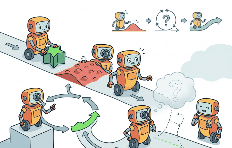
This section assumes familiarity with distribution shift and drift detection from section 53.1, and with open-world adaptation from section 51.4. The governed pipeline introduced here is extended in section 57.2, which addresses catastrophic forgetting as the central technical risk that makes staged rollout necessary, and in section 57.3, which covers replay and regularization strategies for managing it.
A warehouse robot ships with a policy trained on a thousand objects. Six months later, new product lines arrive and pick rates drop 30%. The team wants the robot to learn from field data, but a silent weight update could fix grasping while quietly breaking collision avoidance. No one notices until the first incident report. Embodied systems deployed in the real world will always drift; the question is whether the update loop is governed or improvised. Here you will build the four-stage pipeline that separates monitoring, candidate training, validation, and staged rollout, so adaptation is controlled, auditable, and safe to run continuously.
The update pipeline is part of the embodied system. If the learning loop cannot be audited, then post-deployment improvement is operating outside the same scientific standard demanded of perception, planning, and control.
Theory
A single silent weight update that lifts grasp success by three points can, in the same gradient step, push a collision-avoidance margin below the threshold that keeps a forklift-sized robot from hitting a person, and nothing in the loss curve will warn you. That coupling is why post-deployment learning must be governed like a release pipeline rather than treated as spontaneous self-improvement, and why it should be modeled as a staged pipeline:
$$D_t \rightarrow U_t \rightarrow \theta_{t+1} \rightarrow V_t \rightarrow R_t,$$
where collected field data \(D_t\) feeds an update rule \(U_t\), producing candidate parameters \(\theta_{t+1}\), which are evaluated by validation suite \(V_t\) before rollout decision \(R_t\). The key idea is that deployment data and deployment decisions are connected, but not collapsed into one uncontrolled online loop. Figure 57.1B traces these five stages left to right, including the red rollback path that returns control to monitoring whenever a check fails.
Notice that rollback is the only stage in the pipeline where nothing can go wrong: it just points at the previous version. Every other stage is where engineers spend their weekends.
| Stage | Artifact | Failure If Missing |
|---|---|---|
| Monitoring | drift and intervention report | no justified reason to update |
| Candidate update | versioned training config and data slice | cannot explain what changed |
| Validation | old-task, new-task, and safety panel | silent regressions |
| Rollout | shadow or canary decision log | unsafe direct promotion |
| Rollback | pointer to previous stable version | slow or impossible recovery |
Worked Example
Suppose a shelf-picking robot sees more reflective packaging after a supplier change. The new data may justify a candidate perception update, but only after the system verifies that prior carton and bottle skills still work.
def validate_update_pipeline(payload: dict[str, object]) -> dict[str, object]:
    assert payload, "payload must not be empty"
    return payload

update_pipeline = {
    "field_signal": "drop in grasp success on reflective cartons",
    "candidate_update": "fine-tune perception head on corrected examples",
    "validation_panel": ["old carton tasks", "new reflective carton tasks", "safety replay set"],
    "rollout_mode": "shadow_then_canary",
}
print(validate_update_pipeline(update_pipeline))
{'field_signal': 'drop in grasp success on reflective cartons', 'candidate_update': 'fine-tune perception head on corrected examples', 'validation_panel': ['old carton tasks', 'new reflective carton tasks', 'safety replay set'], 'rollout_mode': 'shadow_then_canary'}validate_update_pipeline asserts the update record is non-empty and echoes back its four required fields, field_signal, candidate_update, validation_panel, and rollout_mode, making an ungoverned retrain fail loudly rather than ship silently.The expected output should make the release logic explicit. If the update pipeline does not name retained-task checks and rollout mode, then "learning after deployment" is really just ungoverned retraining.
A policy that improves in the field without a governed pipeline is not learning: it is drifting with good intentions.
- Detect a field signal such as drift or recurring intervention.
- Create a candidate update from labeled data, replay, or adapters.
- Evaluate old tasks, new tasks, and safety cases in one fixed panel.
- Deploy only in shadow or canary mode first.
- Promote or roll back according to explicit thresholds.
Step-Through: Governed Field Learning on a Pick Robot
Trace the five stages with concrete numbers for a shelf-picking robot after a supplier swaps in reflective cartons. Stage 1, Monitor: grasp success on reflective cartons drops from 0.94 to 0.61 over 2,000 logged picks, crossing the drift alarm threshold of a 0.10 absolute drop, so an update is justified. Stage 2, Candidate: a LoRA adapter (r=8, lora_alpha=16), where LoRA (Low-Rank Adaptation) freezes the original weights and learns only a small pair of low-rank update matrices, is fine-tuned on 1,400 corrected reflective-carton frames, touching 0.5% of parameters; the frozen backbone keeps planning and force-control weights untouched. Stage 3, Validate: the fixed panel reports old cartons 0.93 (was 0.94, within the 0.02 tolerance), new reflective cartons 0.90 (up from 0.61), safety replay 0/512 collisions. All three gates pass. Stage 4, Rollout: shadow mode runs 48 hours; the candidate action stream diverges from production by more than 5 cm on only 0.3% of frames, below the 1% promotion cap, so canary opens on 3 of 40 units, where a canary is a small subset of live units that runs the candidate with real control authority while the rest of the fleet stays on the stable version. Stage 5, Promote or roll back: canary holds 0.90 success and 0 safety events for 72 hours, so the update promotes fleet-wide. Had old-carton success fallen to 0.87 in stage 3, the red rollback path would have fired and the previous stable version would have stayed live.
Real-World Application: Autonomous Vehicle Perception
Tesla's fleet learning loop is typically described as a large-scale governed pipeline: field clips that trigger driver interventions are uploaded, used to train candidate perception networks, and validated against a fixed regression suite of previously logged scenarios before any release. New networks are generally shipped to a small shadow population first, where their predictions are compared against production output on real sensor streams without ever controlling the car, an approach consistent with the monitor-validate-shadow-canary sequence described here, though exact internal thresholds are not publicly documented.
Replay stores, versioned experiment trackers, adapter-tuning libraries, and deployment registries are valuable here because they preserve provenance. The shortcut is helpful only when the tool chain retains old-task panels, candidate lineage, and rollback pointers rather than just storing a new checkpoint.
Teams often let new field data dominate the update pipeline without preserving enough old-task evidence. The result is adaptation that looks good on the latest problem and quietly regresses earlier competence.
A common assumption is that learning after deployment means the robot can update its weights in real time from new experiences, the way a person learns by doing. This assumption is wrong in the embodied AI context. A live weight update changes every behavior the policy controls at once. Fixing a grasping failure can silently degrade collision avoidance, localization, or force control, with no visible error at update time. The correct mental model is a release pipeline: new experience generates a candidate policy, the pipeline validates that candidate against a fixed panel of old tasks and safety cases, and only a passing candidate earns live control authority through shadow or canary stages. Continuous improvement and continuous deployment are two different things. Only the latter is safe without a governed pipeline.
Amazon Robotics' Proteus autonomous mobile robot and the Boston Dynamics Spot inspection fleet both ship perception updates through staged rollout mechanisms rather than live online learning: a candidate model runs in shadow mode alongside the production model for a defined window (often 24 to 72 hours of operational coverage), and promotion requires the shadow model to match or exceed the production model on a fixed set of logged scenarios before any canary release to live units. The staged window is not arbitrary: it is sized to cover the diurnal and shift-change variation in the environment so that a model that only works well on the morning shift cannot pass validation.
A hospital delivery robot that sees new floor reflections after waxing may need a localization update. A governed pipeline first labels the reflective cases, then checks retained hallway navigation and elevator entry, then promotes the update in shadow mode before granting live control authority.
Direction 1: Parameter-efficient continual adaptation for foundation robot policies. Large visuomotor foundation models such as Octo (Octo Model Team, 2024) and pi0 (Black et al., 2024) are being adapted post-deployment via low-rank or modular updates rather than full fine-tuning. Active work at Berkeley RAIL and Physical Intelligence asks which parameter subsets can absorb field distribution shift without corrupting the frozen backbone's generalization, and how safety-validation panels must change when the adapter is the only part that moves.
Direction 2: Online data curation and filtering for deployment loops. As of 2024, the GROOT and AHA lines of work from NVIDIA Research explore automated quality scoring of self-collected robot trajectories so that only interventions and near-failures, not routine successes, enter the update candidate pool. The core insight is that unfiltered field data is dominated by in-distribution successes that add noise rather than signal to a retrained policy head.
Direction 3: Deployment-time task-incremental learning without task labels. Recent work on continual learning for embodied agents (e.g., ConTinual Adaptation for Robots, Carta et al., 2024) removes the assumption that the system knows when a new task boundary has occurred, forcing the pipeline to infer boundaries from field signals alone. Most current governed pipelines assume a human engineer declares a task boundary before triggering an update; lifting that assumption is the focus of several 2024 to 2026 ICLR and CoRL submissions.
Open PhD problem: All three directions above produce candidate policies that are validated offline before any canary release. No current method provides a formal bound on the probability that a candidate policy that passes an offline validation panel will also be safe on hardware for the first 72 hours of canary exposure. Constructing a statistically grounded sample-size prescription for the validation panel, one that accounts for temporal autocorrelation in field data and the gap between simulation and hardware closed-loop dynamics, is an open and tractable PhD-scale problem.
Can you name the field signal, candidate update, retained-task panel, and rollout mode for one real robot application? If any of those are missing, the learning loop is still underspecified.
Naming those four artifacts is the concrete skill this section aims to build: given any post-deployment adaptation scenario, you should now be able to specify what triggers an update, what the candidate change is, what evidence must pass before rollout, and how rollout is staged, which is exactly what the exercise and lab below ask you to practice.
Shadow mode matters for physical robots for a specific reason. A weight change that looks safe in simulation can still destabilize closed-loop dynamics on hardware. Actuator-response latency, sensor quantization noise, and mechanical wear all create edge cases that offline evaluation cannot replicate. Running the candidate policy in parallel, with its outputs logged but not executed, lets the team observe real sensor streams and real object poses without accepting any physical risk from the new weights.
Mechanically, shadow mode runs the candidate model on every live sensor frame alongside the production model. The production model's action is sent to the actuators; the candidate model's action is recorded to a comparison log. After the shadow window closes, engineers diff the two action streams on the scenario panel, checking for divergences above a threshold before any canary promotion begins.
The update record travels with the model
Logging two action streams is only useful if you can later reconstruct exactly which candidate produced them, which is why the comparison artifact has to travel with the rest of the update record. In production systems, the update object is usually larger than a checkpoint. It should include the exact slice of field data, labeling protocol, adapter or fine-tuning configuration, validation manifest, and the deployment ticket that authorized the shadow or canary run. Tools such as PyTorch training jobs, Weights and Biases or TensorBoard traces, and ROS 2 replay logs are useful here only when they preserve this bundle as one inspectable release artifact rather than scattering evidence across unrelated dashboards.
A strong post-deployment recipe also distinguishes perception adaptation from control adaptation. Suppose a warehouse robot fails because carton appearance changed. The first candidate may then be a narrow vision update with frozen planner and controller interfaces. A LoRA adapter on the vision head touches roughly 0.5% of total parameters, so the 99.5% of weights that govern planning and force control cannot move at all, and a fleet-wide risk becomes a strictly bounded one. If the failure instead comes from timing drift or changed vehicle dynamics, the update path may involve different evaluation panels, different rollback rules, and stricter closed-loop replay before any canary release.
Checkpoint
So far: shadow mode lets a candidate policy run silently alongside production to compare action streams without physical risk, the update record bundles that comparison with data, config, and authorization into one inspectable artifact, and splitting perception updates from control updates keeps a narrow fix from putting the whole parameter set at risk.
Before reading on, consider: if you could only keep one of the five pipeline stages when shipping under deadline pressure, which would you drop, and what would you lose?
When updating only a perception head after deployment, use a Low-Rank Adaptation (LoRA) adapter (via the peft library with LoraConfig(target_modules=["q_proj","v_proj"])) rather than full fine-tuning: this freezes the backbone by construction and limits weight drift to the adapter matrices, so the planner and controller interfaces cannot be inadvertently shifted. Set lora_alpha to twice r as a starting point; a ratio below 1.0 often produces adapters too weak to correct real distribution shift, while a ratio above 4.0 tends to destabilize the retained-task panel.
Learning after deployment also reshapes organizational interfaces. Operators, data curators, and release owners need a shared artifact vocabulary so that any update can be challenged and reversed without ambiguity.
Beyond clarifying who can challenge an update, the staged structure also determines whether the update is even tested against the conditions that matter. The staged pipeline matters most when distribution shift is correlated with time of day, seasonal change, or operational context rather than being a random fluctuation. A robot that sees fewer training examples of wet floors in summer will encounter them in winter; if its perception update was triggered only by recent data, the summer model may degrade exactly when wet-floor robustness is most needed. Consider scale: a validation panel covering only the last 7 days of logs may include zero wet-floor encounters, while a panel spanning 90 days typically captures 15 to 40 such cases, enough to detect a regression before promotion. Staging creates a forcing function: the validation panel must be drawn from a distribution that spans known temporal and contextual variation, not just the most recent week. In other words, a panel built only from this week's logs can pass an update that is actually blind to a whole season of conditions; when that panel is narrow, this is called the temporally biased update trap, and the failure will appear as a surprise regression months after the update was promoted.
Think of a ship's navigator who calibrates the compass only on calm days in harbor. The calibration looks perfect against every reading taken during those sessions, but the instrument has never been checked in a storm, when magnetic interference from the engine room peaks. The ship sails fine all summer, then one winter night the compass gives a steady, confident reading that is six degrees off, and no one suspects it because the calibration log shows only green. A validation panel built from the last seven days of logs is the same compass: it passes on the conditions that happened to occur this week, and fails silently on the conditions that have not come around yet.
Learning after deployment is a governed release process, not a permission slip for uncontrolled online adaptation.
Project Ideas
Drift detector for a simulated warehouse robot (beginner, weekend): Use Gymnasium with a custom wrapper that periodically swaps object textures mid-episode to simulate a supplier change, then log grasp success rate over time to detect the shift automatically. The key challenge is choosing a detection threshold that fires on real drift without triggering false alarms from normal variance in a short episode window.
Governed fine-tuning pipeline for a manipulation policy (intermediate, 1-2 weeks): Train a base pick-and-place policy in Isaac Lab or MuJoCo (as of 2024, PyBullet is in maintenance mode and Isaac Lab is the preferred GPU-accelerated alternative), collect simulated field failures by degrading lighting conditions, fine-tune a LoRA adapter on the failure cases using the peft library, and gate promotion behind a validation panel that replays the original task suite before accepting the update. The key challenge is constructing a retained-task panel that spans enough temporal and contextual variation to catch regressions that would only appear after promotion.
Lab: Catch a Silent Regression with a Validation Gate
Goal: feel the temporally biased update trap firsthand by training a classifier, "deploying" an update, and watching it pass a narrow validation panel while quietly regressing on conditions the panel never sampled.
Tools needed: Python, scikit-learn, and NumPy (15 to 30 minutes). Use a two-class image or tabular task (for example, MNIST split into digits-with-noise vs. clean digits) where you can deliberately add a "lighting condition" by injecting Gaussian noise of varying intensity into a subset of samples.
Procedure: (1) Train a base model on low-noise data only. (2) Simulate field drift by fine-tuning on a new high-noise slice that mimics a recent supplier change. (3) Build two validation panels: a narrow one drawn only from the last "week" (high-noise samples) and a broad one spanning all noise levels. (4) Gate promotion on each panel in turn.
What to vary: the noise intensity of the field slice, the fraction of old-condition samples in the narrow panel (start at 0%), and the promotion threshold. What to observe: the narrow panel approves an update whose accuracy on clean, low-noise inputs has collapsed, while the broad panel blocks it. Plot accuracy per noise level before and after the update to see exactly where the silent regression hides.
Design a field-learning pipeline for a mobile robot whose localization degrades in reflective hallways. Name the field signal, candidate update, retained-task panel, and rollout mode.
Section References
Kirkpatrick, J. et al. Overcoming catastrophic forgetting in neural networks. PNAS, 2017.
Use for regularization-based retention and its assumptions.
Lopez-Paz, D. and Ranzato, M. Gradient Episodic Memory for Continual Learning. NeurIPS, 2017.
Use for replay-constrained updates and task-stream evaluation.
What's Next?
Next, continue with Section 57.2, where the main technical risk becomes catastrophic forgetting.