Section 4.5: 2D and 3D transformations; transform trees (tf in ROS)

"Every joint has its own truth about where things are. The transform tree is how the robot reconciles them all without asking anyone to agree."

A tf Listener, Querying at Time Now

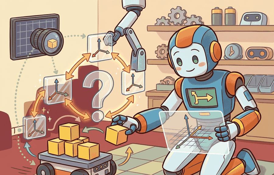
A surgical robot threading a needle, a warehouse forklift placing a pallet, and a humanoid catching a thrown ball all share one quiet dependency. At every instant each must answer "where is that thing in the frame my actuator controls?" It must answer from a graph of named coordinate frames rather than a drawer of hardcoded offsets. Figure 4.5A above shows the shape of what we are building: a transform tree for a mobile manipulator. Its world-to-odom, odom-to-base, base-to-arm, and camera edges let a tf lookup resolve between any pair of frames at a given timestamp. The technical contract for 2D and 3D transforms is a graph problem. A transform tree is a directed acyclic frame graph with one parent per child. A lookup composes edges along a path. The math then maps onto the ROS tf2 discipline of stamped transforms, buffer windows, and explicit lookup times. A robot that cannot name where each frame sits relative to every other frame does not have a coordinate problem; it has a knowledge problem, and the transform tree makes that knowledge queryable.

The key question is practical: when a camera detects an obstacle, which chain of transforms converts that obstacle into the planning frame at the time the planner needs it?

This section builds that answer in three concrete deliverables so the promise above is not left abstract: a lookup algorithm you can implement (the Transform-Tree Path Lookup box), a worked composition from map to camera you can trace by hand (Code Fragment 4.5.1 and the Step-Through), and the specific tf2 usage rules that make the algorithm work correctly in ROS (stamped queries, static versus dynamic broadcasters, and buffer timeouts, covered in the Mechanism, Library Shortcut, and Failure Modes boxes below).

Theory

A transform tree stores edges such as \(T_{\text{map},\text{odom}}\), \(T_{\text{odom},\text{base}}\), and \(T_{\text{base},\text{camera}}\). A lookup from camera to map follows the unique path through the tree and composes the transforms in path order:

$$T_{\text{map},\text{camera}} = T_{\text{map},\text{odom}}T_{\text{odom},\text{base}}T_{\text{base},\text{camera}}.$$

This is why tf2 insists on parent and child frame names. Without the names, a transform matrix is only a 4 by 4 array. With the names and timestamp, it becomes a claim about where one coordinate convention sits relative to another at a specific time.

2D transforms are the same idea with fewer degrees of freedom. A planar robot often uses \((x, y, \theta)\) and the group SE(2) (Special Euclidean group in two dimensions). A flying robot, manipulator, or camera-bearing humanoid needs SE(3) (Special Euclidean group in three dimensions), because roll, pitch, yaw, and vertical translation are load-bearing state variables. Choosing SE(2) when the robot actually tilts is not a modelling simplification: it is a silent accuracy failure. A wheeled robot on uneven terrain may roll 3 to 5 degrees, which projects a camera target 30 cm overhead into the wrong floor-plane position by several centimetres. At grasping tolerances that error is the difference between a successful pick and a dropped object. Before reading on, ask yourself: if upgrading from SE(2) to SE(3) costs almost nothing on a modern CPU, why do so many real deployed systems still use planar transforms for 3D robots? The answer is usually inertia combined with the fact that the failure is silent. The system works on flat floors in the lab, ships, and then drops objects the first time it encounters a loading dock ramp.

Since that failure is purely a matter of which group you store each edge in, it helps to see exactly how little the two representations differ on disk. Mechanically, SE(2) represents a transform as a 3 by 3 matrix with one rotation angle and two translation components; SE(3) uses a 4 by 4 matrix with a 3 by 3 rotation block and a 3-vector translation. Upgrading a tf2 edge from SE(2) to SE(3) means storing three additional rotation parameters per edge and composing with 4 by 4 matrix multiplication instead of 3 by 3, a cost that is negligible on modern CPUs but requires consistent type discipline across every node that publishes or consumes that edge. That per-edge type discipline pays off only because the tree turns every edge into a shared resource, which is where its real advantage over scattered calibration files emerges. The decisive advantage over per-subsystem calibration files is composability under change. Mounting a new sensor adds exactly one edge. Every consumer that queries through that sensor's frame gets the correct composed result at once, with no downstream code changes.

Why the tree wins at scale

Consider the scale, illustratively: the figures below are a representative hypothetical, not a measurement from one deployment. A humanoid robot with 30 joints, 4 cameras, a lidar, and an IMU (Inertial Measurement Unit) needs 38 edges in its transform tree. Without the tree, each of 12 perception modules hardcodes and maintains its own path through those 38 relationships. That produces up to 456 places where a single sensor remount could cause silent errors. With the tree, the same remount is one edge update. Compare the two recovery paths after a camera recalibration at a busy warehouse deployment. Without the tree, a team can easily spend two days coordinating across groups to patch every downstream module. With the tree, an engineer edits one URDF line (URDF is the Unified Robot Description Format, the XML file that declares a robot's frames and their fixed offsets) and restarts the static broadcaster, a change measured in minutes. The tree also enforces discipline that a direct static matrix cannot provide. Frame names make direction explicit. Timestamps make the query time explicit. The parent-child invariant prevents loops. A system that hardcodes \(T_{\text{base},\text{camera}}\) directly into the perception node breaks the moment that sensor moves or the robot gains a second camera. The tree absorbs both changes with a single edge update. This design is called the one-edge principle: any physical reconfiguration touches exactly one entry in the graph.

Worked Example

Code Fragment 4.5.1 implements the smallest useful transform-tree lookup. It stores three edges, composes the path from map to camera, and applies the resulting transform to one point reported by the camera.

# Compose a tf-style path from map to camera and transform one point.
# Each edge is named by parent and child frame to prevent silent direction bugs.
# The example omits rotation so the path arithmetic is easy to inspect.
import numpy as np

def translate(x, y, z):
    transform = np.eye(4)
    transform[:3, 3] = [x, y, z]
    return transform

edges = {
    ("map", "odom"): translate(2.0, 0.0, 0.0),
    ("odom", "base_link"): translate(0.5, 1.0, 0.0),
    ("base_link", "camera"): translate(0.2, 0.0, 0.8),
}

path = [("map", "odom"), ("odom", "base_link"), ("base_link", "camera")]
map_from_camera = np.eye(4)
for edge in path:
    map_from_camera = map_from_camera @ edges[edge]

point_camera = np.array([1.0, 0.0, 0.0, 1.0])
point_map = map_from_camera @ point_camera
print(point_map[:3].round(3).tolist())

Expected output: the point moves by the sum of the three translations. If a real tf2 lookup gives a different direction, inspect whether the code requested source-to-target or target-to-source, and whether the lookup time matches the sensor timestamp.

Transform-tree bugs look like weak perception or control. Check parent-child direction, timestamp, static-vs-dynamic classification, and buffer latency before changing the robot policy.