"The fastest robot lesson is the one learned before the robot hits the table."
A Safety-Cased AI Agent
This section assumes familiarity with the agent-environment boundary introduced in section 2.1 and the observation-action loop formalized in section 2.3. The cost arguments here are extended in section 9.2, which separates simulation's roles as data generator, testbed, and curriculum. The sim-to-real gap (the mismatch between a simulator's physics and the real hardware's physics, which causes a policy that succeeds in simulation to underperform or fail on the physical robot) that makes hardware trials necessary is analyzed in depth in section 13.2 (domain randomization) and section 20.1 (sim-to-real transfer).
A robot arm attempting to learn a new grasp policy (a function mapping each sensor observation to a motor action through the observation-action loop) from scratch on real hardware needs roughly 10,000 trials. At two minutes per attempt, including resets, that is three weeks of continuous operation, plus operator time, plus the cost of whatever it drops. This is not an edge case; it is the baseline tax on any embodied learning loop. Modern simulation changes that arithmetic by orders of magnitude, and understanding exactly why matters now: the field is reaching the point where policies trained largely or entirely in simulation are, in practice, being deployed on physical systems in warehouses and factories, with hospital and home deployments still comparatively rare and typically confined to narrower, more constrained tasks. By the end of this section you will be able to quantify the hidden costs of real-world training and explain precisely where simulation earns its place in the pipeline.
A policy trained only on hardware is not a policy shaped by evidence; it is a policy shaped by whatever the hardware happened to survive.
The Real Cost Of Learning By Doing
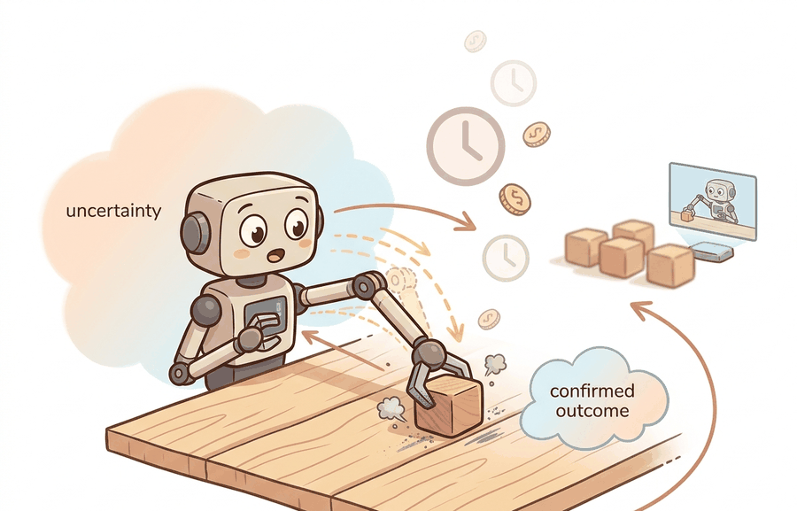
Figure 9.1A makes the gap visible: time per episode, repair cost per crash, and human supervision hours all stack up on real hardware while a simulation baseline runs the same policy at roughly 1000x speed. A real robot trial has hidden costs: setup time, operator attention, reset time, safety review, calibration drift, wear, and the opportunity cost of occupying the platform. Those costs compound when a policy needs thousands or millions of transitions. Even a small desktop robot becomes a bottleneck if each failed grasp requires a human reset.
Those stacked costs assume the hardware stays consistent across trials, but a second, quieter hazard erodes that assumption from underneath: calibration drift. This section introduces calibration drift here as a cost category; the Real-World Training Feasibility Decision Checklist later in this section (steps 7 and 8) gives the procedure for detecting and budgeting it before a policy reaches hardware, so the mechanism below is worth holding onto.Calibration drift matters because a robot's learned policy encodes the sensor and actuator characteristics present at training time. When joint encoders, force-torque sensors, or cameras shift from their calibrated baseline, the policy receives observations that no longer match its training distribution. Performance then degrades without any obvious failure signal. Embodied AI treats this as a baseline hazard, not a corner case. Prolonged operation causes thermal expansion, gear wear, and cable stretch. Each effect shifts sensor readings by small amounts that a single session can hide. Across weeks of trials, though, those shifts grow large enough to break a precision grasp policy.
The mechanism is a mismatch between the internal world model embedded in the policy and the actual physical state of the hardware, a gap that opens precisely at the agent-environment boundary. The policy maps an observation vector to an action. If the encoder reporting joint angle has drifted by two degrees, every grasp attempt will be offset by that error, consistently and silently. Detecting drift requires periodic recalibration runs against a known reference pose, comparing live sensor readings to a stored baseline and recomputing offset tables before resuming policy evaluation.
Think of calibration drift like a kitchen scale that slowly loses its zero over weeks of use. Every recipe you follow uses the same instructions, but if the scale reads two grams heavy, every measurement is consistently wrong by that amount without ever showing an obvious error. A grasp policy experiencing encoder drift is in the same position: its internal recipe is correct, but the measurements feeding it are silently offset, so every reach lands in the wrong place by a fixed, invisible margin. The only fix is to re-zero the scale against a known weight, which in robotics means running a calibration sequence against a reference pose before trusting the policy again.
Simulation matters because it changes the economics of hypothesis testing: a simulated rollout costs microseconds and zero risk, while a real hardware trial costs minutes, operator attention, and a non-zero chance of damage. To make the scale concrete: a reward function that turns out to be exploitable will reveal itself in roughly 300 simulated episodes; catching the same flaw on a physical arm, at two minutes per episode plus reset, would consume 50,000 episodes and nearly 70 days of continuous operation. A simulated rollout can reject an unstable reward, unsafe action range, brittle controller, or bad observation design before the first hardware trial. The goal is not to avoid reality. The goal is to arrive at reality with sharper hypotheses.
Simulation is central when it moves avoidable mistakes away from hardware and into a falsifiable rehearsal space. Real trials should measure the assumptions that simulation could not settle.
| Cost | What It Means | Why Simulation Helps |
|---|---|---|
| Reset time | Returning the world to a clean initial state | Simulators reset thousands of worlds without a human operator |
| Safety exposure | Collisions, dropped objects, overheated motors, and unsafe motion | Unsafe actions can be bounded and rejected before hardware |
| Coverage | Rare layouts, lighting, friction, and object poses | Randomization can sample edge cases that real collection rarely reaches |
| Debug latency | Time between a failure and a diagnosis | State, contacts, seeds, and policy decisions can be replayed exactly |
Worked Miniature: A Trial Budget
Code Fragment 9.1.1 turns this intuition into a trial ledger. The point is not the exact numbers. The point is that every physical learning loop should expose its time, cost, and risk budget before a policy is trained.
# Estimate the hardware budget before choosing a training loop.
# The calculation makes reset time and safety exposure visible.
trials = 200_000
action_seconds = 2.0
reset_every = 10
reset_seconds = 20.0
operator_cost_per_hour = 45.0
risk_events_per_1000 = 1.5

action_hours = trials * action_seconds / 3600
reset_hours = (trials / reset_every) * reset_seconds / 3600
total_hours = action_hours + reset_hours
operator_cost = total_hours * operator_cost_per_hour
expected_risk_events = trials / 1000 * risk_events_per_1000

print({
    "hardware_hours": round(total_hours, 1),
    "operator_cost_usd": round(operator_cost, 0),
    "expected_risk_events": round(expected_risk_events, 1),
})
{'hardware_hours': 222.2, 'operator_cost_usd': 10000.0, 'expected_risk_events': 300.0}Step-Through: Trial Budget Ledger
Trace the ledger with a tiny example. Suppose you only need 1,000 trials, each action takes action_seconds = 2.0, you reset once every reset_every = 10 trials, each reset takes reset_seconds = 20.0, the operator costs $45/hour, and the platform produces risk_events_per_1000 = 1.5. Step 1, action time: 1000 x 2.0 = 2000 seconds, divided by 3600 = 0.556 hours. Step 2, reset time: 1000 / 10 = 100 resets, times 20.0 = 2000 seconds, divided by 3600 = 0.556 hours. Step 3, total hardware time: 0.556 + 0.556 = 1.11 hours. Step 4, operator cost: 1.11 x 45 = $50. Step 5, expected risk events: 1000 / 1000 x 1.5 = 1.5 events. Even this miniature run already predicts more than one likely safety event, which is exactly the signal that says push exploration into simulation. Notice that resets contribute as much wall-clock time as the trials themselves, a cost that is invisible until you write it down.
Expected output: the ledger shows that 200,000 exploratory steps would occupy about 222 hardware hours, cost roughly $10,000 in operator time, and expose the system to hundreds of expected risk events. Those numbers motivate moving broad exploration into simulation while reserving real trials for calibration and transfer checks.
Consider a specific case. The Dexterous In-Hand Manipulation work from OpenAI (Andrychowicz et al., 2020) trained a policy entirely in MuJoCo with domain randomization (deliberately varying simulated physical parameters such as mass, friction, and lighting across training runs so the policy learns to tolerate the kind of variation it will meet on real hardware) across 128 parallel simulation workers. That run accumulated roughly 100 years of simulated experience before a single hardware trial. Dactyl is the name OpenAI gave the physical five-fingered robot hand used for the hardware trials. Evaluation and fine-tuning then needed about 50 real Dactyl robot hours. At the ledger numbers above, 100 simulated years would have cost tens of millions of dollars and an impractical number of resets on physical hardware. Simulation did not replace the real robot; it changed what the real robot was used for, narrowing its role to measuring assumptions the simulator could not settle (contact deformation, tendon compliance, camera latency).
About 18 lines of accounting become a structured experiment budget in tools such as MuJoCo, Isaac Lab, and ManiSkill, where reset frequency, episode length, random seeds, and failure categories can be logged automatically. The hand ledger remains useful because it forces the team to name the real-world cost that simulation is meant to reduce.
What Simulation Can Falsify
Once the ledger has justified moving exploration off hardware, the next question is what that cheap exploration can actually establish, and the honest answer is that simulation proves nothing but rejects a great deal. A simulator cannot prove that a policy will work in reality. It can falsify many reasons the policy should not be trusted yet. It can show that the action range is unstable, the reward is exploitable, the controller saturates, the perception stack depends on privileged state, or the policy succeeds only for one seed and one friction value.
Before running a single hardware trial, ask yourself: if the policy fails on the real robot, will you know why it failed, or will you just know that it did?
Algorithm: Real-World Training Feasibility Decision Checklist
Input: Task description, hardware platform, policy class \(\pi_\theta\), candidate reward \(r(s, a)\), allowed trial budget \(B\)
Output: Decision: train in simulation, train on hardware, or use mixed curriculum; flagged risk categories
- Estimate the real-world trial budget: compute hardware hours \(T = N \cdot t_\text{step} + \lfloor N / k \rfloor \cdot t_\text{reset}\), where \(N\) is the target number of transitions, \(t_\text{step}\) is average action duration, \(k\) is episode length, and \(t_\text{reset}\) is mean reset time. If \(T \gt B\), flag as hardware-infeasible.
- Audit the action space: verify that every \(a \in \mathcal{A}\) satisfies velocity, torque, and collision constraints. If the space contains unbounded or untested regions, mark exploration as unsafe for hardware until bounds are confirmed in simulation.
- Inspect the reward \(r(s, a)\): check whether it depends on privileged simulator state not available on hardware (ground-truth contact forces, exact joint positions, zero-latency resets). Any such dependency disqualifies the reward from direct hardware use.
Checkpoint
So far: the checklist has covered three checks, whether the trial budget fits the hardware hour allowance, whether the action space is bounded and safe, and whether the reward secretly depends on information the real robot cannot observe. The remaining steps below shift from budget and safety checks to policy stability, failure diagnosis, and transfer readiness.
- Probe policy stability: run the current policy \(\pi_\theta\) under at least five random seeds and two perturbation levels \(\delta\) applied to initial state \(s_0\). If return variance \(\text{Var}[G] \gt \epsilon_\text{thresh}\), the policy is not stable enough for hardware trials.
- Run a deliberate failure probe: deploy the weakest reasonable baseline that should fail, and verify it fails for a diagnosable reason (perception error, planning error, control saturation). If failure mode is unclear, do not advance to hardware.
- Check the observation pipeline: confirm that every input \(o_t\) is available from real sensors with known latency \(\Delta t\). Observation components present in simulation but absent or noisy on hardware (privileged state, perfect segmentation) must be replaced before transfer.
- Quantify the reset cost on hardware: if a failed episode requires human intervention, equipment repositioning, or safety inspection, assign a safety-event probability \(p_\text{risk}\) and compute expected events \(E[\text{events}] = N \cdot p_\text{risk}\). If \(E[\text{events}] \gt 1\), constrain exploration to simulation until \(p_\text{risk}\) is reduced.
- Identify simulator-only assumptions: list physical properties (contact stiffness, motor latency, sensor noise \(\sigma\)) that the simulator holds fixed. Each uncovered property is a sim-to-real gap that requires a real calibration measurement before the policy is transferred.
- Assign each unresolved question to its cheapest evidence source: budget questions and coverage questions go to simulation; calibration questions and timing questions go to a short real hardware sequence.
- Record the decision and its rationale as a falsifiable hypothesis: state which simulator assumptions, if violated on hardware, would invalidate the simulated result. Use this record as the transfer checklist in section 13.2.
- Run the simplest policy that should fail, then verify that it fails for the right reason.
- Run the intended policy across held-out seeds, object poses, and perturbations.
- Log failures as perception error, state-estimation error, planning error, control error, simulator mismatch, or metric error.
- Promote only construct-matched, co-computed positive results into paper-facing claims.
A simulator run becomes evidence only after the falsifiable hypothesis, held-out seeds, perturbation panel, and untested real-world assumption are written down.
A common assumption is that the core obstacle to real-world learning is speed, and that adding more robots or automating resets will close the gap with simulation. This is wrong in the embodied AI context because the fundamental constraint is not throughput but irreversibility: a physical robot exploring an unsafe action range can damage hardware, injure bystanders, or corrupt the very sensors needed for calibration, and no amount of parallelism removes that risk during early, unconstrained exploration. The correct mental model treats real-world trials as a scarce and irreplaceable measurement resource, not a slow data pipeline. Simulation's role is to screen out policies that are still unsafe or unstable before they ever touch hardware, so that each real trial tests a specific and already-bounded hypothesis rather than performing blind exploration.
Do not treat simulation as permission to ignore safety. Unsafe action spaces, unbounded velocities, and collision-rich exploration should be constrained in simulation first, then bounded again before hardware trials.
Simulation can hide the very costs it is meant to expose. Three failure modes appear repeatedly in practice. First, a policy that exploits a simulator artifact (frictionless floors, zero sensor noise, instant resets) can appear to solve the task while depending on conditions that never exist on hardware. Second, dynamics randomization narrows the sim-to-real gap but does not close it: if the randomization distribution does not cover the real system's contact stiffness or motor latency, the transferred policy degrades silently. Third, because simulated resets are free, researchers sometimes run far more exploration than the real task actually needs, producing policies that are overfit to the simulator's reset distribution rather than calibrated to the start states the hardware will actually encounter.
A lab with one robot arm can run a short real calibration sequence, estimate reset and failure costs, and use simulation for broad exploration. The real robot then becomes a measurement device for specific hypotheses rather than the default source of every exploratory transition.
If a simulated policy knocks over a virtual lamp, the lab learns something. If the real robot does it, the lab also learns who ordered the replacement lamp.
Active directions (2024-2026):
1. Foundation models as simulation-free policy initializers. Large visuomotor models pre-trained on internet-scale video (e.g., pi0 from Physical Intelligence, 2024) reduce the number of real demonstrations needed by one to two orders of magnitude, shifting the cost question from "how many simulated rollouts?" to "how few real demonstrations can bootstrap transfer?" This directly challenges the assumption that broad exploration must happen in simulation.
2. Automated real-to-sim gap estimation. Rather than hand-tuning domain-randomization ranges, recent work (e.g., RialTo from Columbia/Berkeley, 2024) reconstructs a digital twin from a short real video sequence and automatically identifies which physical parameters are out of distribution, so each simulated training run targets a measurable residual gap rather than a heuristic randomization range.
3. Passive real-world data as a simulation substitute. Projects such as DROID (Stanford, 2024) and Open X-Embodiment aggregate passive teleoperation logs across many labs. Policies co-trained on these logs and simulated rollouts show that unstructured real data can replace a significant fraction of unsafe exploratory simulation, reopening the question of when simulation's cost advantage actually dominates.
Open problem for a PhD student: Given a fixed real-hardware budget (e.g., 10 robot-hours), how should a system dynamically decide, at every training step, whether the next transition should come from simulation or from real hardware, based on the current estimate of simulator model error? No principled adaptive allocation policy exists that jointly accounts for model error, safety exposure, and transfer performance on a held-out physical evaluation.
List the reset time, likely hardware failure, human supervision need, and safety boundary for one embodied task you care about. If any of those are unknown, simulation planning should start with measurement, not training.
Tie the Cost Argument to a Contract
The cost argument pays off only when it is tied to a closed-loop contract: one that names the observation stream, the state estimate, the action representation, the timing budget, and the evaluation artifact. Skip that contract, and a model looks capable in a notebook yet fails the first time a sensor drops a frame or a controller saturates.
Separate the conceptual claim, the systems claim, and the evidence claim. A plausible mechanism, a clean interface, and a closed-loop result are different claims; the section should keep their evidence separate.
| Tool or Library | Role in Reducing Real-World Cost | Builder Advice |
|---|---|---|
| MuJoCo | Physics simulation for robot arms and dexterous hands; used in Andrychowicz et al. (2020) to accumulate 100 simulated years on 128 workers before a single Dactyl trial | Set mjModel.opt.timestep to 2ms for contact-rich tasks; coarser steps (5ms) miss finger-tip bounce dynamics and degrade sim-to-real transfer on the Franka Panda. |
| Isaac Lab (NVIDIA) | GPU-vectorized simulation for legged robots and mobile manipulators; runs thousands of parallel Spot or ANYmal environments to compress real wall-clock time from weeks to hours | Use InteractiveScene with ArticulationCfg for a physical robot's URDF; log contact_forces and joint_pos_rel from the start so the same signals are available from real hardware sensors on transfer. |
| LeRobot (Hugging Face) | Standardized dataset and training pipeline for imitation learning on low-cost arms (SO-100, Koch v1.1); provides real hardware teleoperation data alongside simulated rollouts so the cost gap is directly measurable | Compare episode cost in lerobot/common/datasets/lerobot_dataset.py against the trial ledger above; a LeRobot real episode costs roughly 2 minutes of teleoperation plus reset, while a simulated Action Chunking with Transformers (ACT) rollout in gym-pusht runs at roughly 300x real time on a modern GPU (as of 2024). |
| ROS 2 + ros2_control | Exposes real hardware latency and sensor jitter that simulation hides; running the same policy node against a Franka Panda via franka_ros2 immediately reveals the 1ms command round-trip and the 8ms joint-state publish period that MuJoCo masks | Time-stamp every observation with rclpy.time.Time and compare against simulation logs; latency differences above 5ms between sim and real typically cause policy degradation in high-speed contact tasks. |
| Gymnasium (Farama) | Standard reset() and step() interface that makes simulated reset cost explicit; wrapping a real robot arm in a gymnasium.Env subclass forces the team to measure reset time and expose it in info alongside the simulated baseline | Override reset() to log wall-clock time; the difference between a simulated reset (microseconds) and a real hardware reset (20 to 60 seconds for a Franka returning to home pose) is the core cost argument in this section made concrete. |
Start with a small baseline that logs inputs, outputs, units, timestamps, and termination conditions before moving to Gymnasium or PettingZoo. The library run should keep the same artifact schema, so the comparison remains a same-task evaluation.
- Write a one-paragraph task contract with observation, action, success, and failure fields.
- Start with the smallest simulator, dataset, or wrapper that exposes the task contract faithfully.
- Run one deterministic smoke test and one perturbation test before scaling.
- Save a single result artifact containing configuration, seed, metrics, videos or traces, and failure labels.
- Compare methods only when one script evaluates them on the same task panel.
When an experiment about why real-world learning is slow, costly, and risky fails, avoid labeling the whole method as weak. First assign the failure to perception, state estimation, planning, control, timing, data coverage, or evaluation. Then rerun one controlled perturbation that isolates the suspected cause. This pattern turns a disappointing rollout into a reusable diagnostic asset.
Real-World Application: Warehouse Manipulation
Covariant (now part of Amazon) reportedly built its warehouse picking robots by training grasp policies largely in simulation across a broad range of synthetic object arrangements before deploying to live distribution centers. Exact training figures are not independently published, so the scale described here should be read as an industry-reported order of magnitude rather than a verified count. In practice, the physical robots are then reserved for measuring the residual gap (suction failures on deformable packaging, lighting changes on shiny barcodes) rather than for blind exploration, illustrating the slow-costly-risky tax this section quantifies.
Lab: Measure the Hidden Reset Tax
Goal: Empirically confirm that reset time, not just action time, dominates the cost of a real-style learning loop. Tools: Python 3, gymnasium, and the time module (15 to 30 minutes). Steps: Wrap gymnasium.make("CartPole-v1") and run 5,000 episodes of a random policy, timing each env.reset() and the full episode separately with time.perf_counter(). Sum the two totals. What to vary: add an artificial time.sleep() inside a reset wrapper to model a real hardware reset (try 0s, 5s, 20s, 60s, matching a Franka returning to home pose), and vary episode length by changing the termination threshold. What to observe: plot total wall-clock against reset delay. You should see the reset term overtake the action term as soon as the simulated reset cost approaches real hardware values, reproducing the ledger result from Code Fragment 9.1.1 with live measurements rather than assumed constants.
Simulation earns its place when it reduces unsafe, slow, or uninformative real-world exploration while preserving the evidence needed for transfer.
Returning to the three costs named in this section's title: slowness was quantified by the trial ledger (hardware hours per policy), cost was quantified by operator dollars in that same ledger, and risk was quantified by expected safety events per trial batch. Simulation does not erase any of the three; it moves most of the exploration that would incur them into a space where they are cheap to test and safe to fail.
For a mobile robot navigation task, estimate the real-world cost of collecting 50,000 exploratory steps. Then specify which part of that collection should move to simulation and which real measurements must remain.
Project Ideas
Beginner (weekend): Build a trial-cost calculator in Python using Gymnasium that wraps a simulated CartPole or Pendulum environment, logs real wall-clock reset time per episode, and prints a cost ledger comparing simulated throughput to a hypothetical hardware loop at $45/hour operator cost. The key challenge is making the reset overhead visible rather than hidden inside the environment abstraction. Intermediate (1 to 2 weeks): Use PyBullet or MuJoCo to train a simple pick-and-place policy on a tabletop arm (Kuka IIWA or Franka Panda URDF), then port the same policy node to a ROS2 interface using ros2_control and measure how contact latency and joint-state publish delay degrade success rate compared to simulation. The key challenge is aligning the observation timestamps between the MuJoCo step clock and the ROS2 sensor stream so the performance gap is attributable to physics mismatch rather than timing artifacts. Advanced (2 to 4 weeks): Reproduce a small-scale version of the Andrychowicz et al. dexterous manipulation pipeline using Isaac Lab: train a two-finger pinch-grasp policy across 64 parallel environments with randomized object mass and friction, log the simulated episode budget, and evaluate the transferred policy on a LeRobot SO-100 arm using the LeRobot dataset pipeline to compare real versus simulated success curves. The key challenge is designing a domain-randomization range that is wide enough to cover real hardware variance without making the simulated task so hard that the policy never converges.
Section 9.2 separates simulation's roles as data generator, testbed, curriculum, and counterfactual probe.
This work shows how randomized dynamics can train policies that tolerate physical mismatch. It is a useful bridge from this chapter into later transfer and domain randomization chapters. Readers should connect this source to why real-world learning is slow, costly, and risky when deciding what is reusable, what is benchmark-specific, and what must be remeasured.
Brockman, G. et al. (2016). "OpenAI Gym." arXiv.
The Gym paper explains the environment API that shaped modern reinforcement-learning experimentation. Readers should use it to understand why reset, step, render, and reward contracts became standard research infrastructure. Readers should connect this source to why real-world learning is slow, costly, and risky when deciding what is reusable, what is benchmark-specific, and what must be remeasured.
This paper anchors the simulator design lineage behind much modern robot learning. It is useful here because it explains why fast, controllable simulation became central to model-based control and policy testing. Readers should connect this source to why real-world learning is slow, costly, and risky when deciding what is reusable, what is benchmark-specific, and what must be remeasured.
Farama Foundation. "Gymnasium Documentation."
Gymnasium is the maintained successor interface for single-agent reinforcement-learning environments. It matters in this chapter because simulation evidence depends on reproducible environment boundaries and seed handling. Readers should connect this source to why real-world learning is slow, costly, and risky when deciding what is reusable, what is benchmark-specific, and what must be remeasured.
NVIDIA. "Isaac Lab Documentation."
Isaac Lab documents a modern robot-learning workflow on top of Isaac Sim. Practitioners should read it when simulation must include vectorized tasks, assets, sensors, and learning-library integration. Readers should connect this source to why real-world learning is slow, costly, and risky when deciding what is reusable, what is benchmark-specific, and what must be remeasured.