Section 29.4: Mapping and occupancy grids

"A grid cell is a decision about where the robot may spend risk."

A Loop Closure That Came Back With Receipts

Problem First

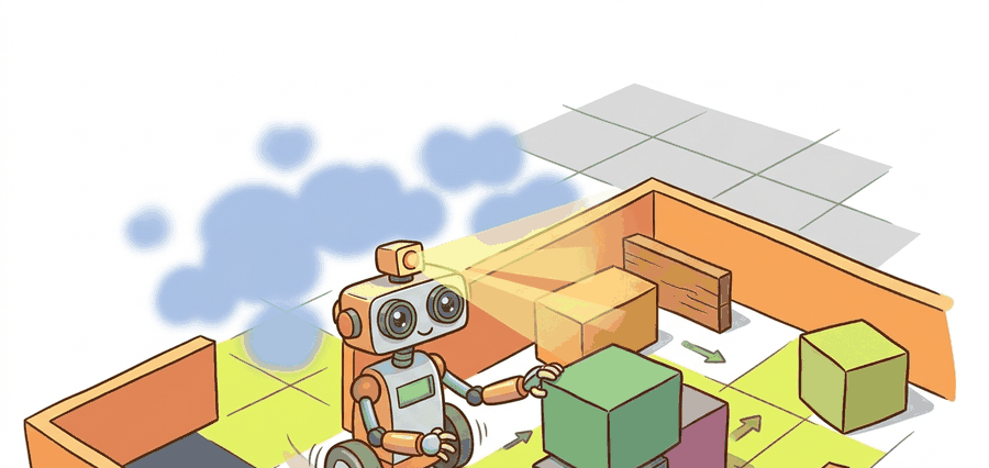
Ask a robot the difference between a hallway it scanned and found empty and a hallway it has never looked down, and a bad map gives the same answer for both: "free." That single confusion is how robots drive confidently into walls they were never told about. A robot map is a probabilistic memory of what sensor rays have implied, tying each cell to a state variable, an uncertainty model, and the next action the robot might take, as Figure 29.4.1 illustrates. Free space, occupied space, and unknown space must stay distinct because a planner should treat unseen cells differently from cells observed as empty. A map that cannot distinguish between "definitely empty" and "never checked" is not a map: it is a wish.

Keeping those three states distinct is not a labeling convention but a consequence of how each cell is updated. Occupancy grids update each cell through inverse sensor models, often using log odds for numerical stability. A range ray decreases occupancy probability along free cells and increases it near the measured endpoint. The map is therefore a belief field, not a bitmap.

The inverse sensor model matters in embodied AI because a physical sensor reports a distance, not a cell state. Without a principled translation from "ray returned at 3.2 m" to per-cell probability changes, the robot either treats every unobserved cell as free (crashes into unmapped walls) or refuses to plan through any unseen space (freezes in novel environments). On a resource-constrained mobile platform, the model also sets the computational budget: a simpler beam model costs microseconds per ray while a more accurate but expensive model stalls the 10 Hz planning loop.

From ray to per-cell probability

The model treats the sensor ray as a likelihood function over grid cells. Consider a LiDAR (Light Detection and Ranging) return at range \(r\). Cells along the ray closer than \(r\) receive a small negative log-odds increment as evidence of free space. The cell at range \(r\) receives a larger positive increment as evidence of an obstacle. Cells beyond \(r\) stay unchanged, because the ray carries no information about them. The sensor's known false-positive and false-negative rates set these increments, so the update follows directly from hardware characterization rather than a hand-tuned heuristic.

Formal Model

To honor that action contract, the informal "belief field" picture needs a precise posterior to update. For occupancy grids, the posterior is a cell-wise belief over free, occupied, and unknown space conditioned on sensor rays and the robot pose estimated by localization. The planner consumes inflation, freshness, and uncertainty, not only a black-and-white bitmap.

$$ L_t(c)=L_{t-1}(c)+\log\frac{p(c\mid z_t,x_t)}{1-p(c\mid z_t,x_t)}-L_0(c) $$

The evidence terms are inverse sensor model, ray casting, pose uncertainty, update rate, decay policy, and map resolution. Each one changes whether a cell is safe to traverse or only looks safe in a stale grid.

Before reading on, guess: if a robot scans a doorway ten times and each scan returns "free," how many occupied-endpoint hits does it take to flip that cell back above 50% occupancy? In practice this number surprises many readers on first encounter, and the log-odds math below shows exactly why.

Consider a specific case: a LiDAR ray 4 meters long hits a wall. The inverse sensor model assigns log-odds of roughly -0.4 to each of the 39 free-space cells the ray passes through, and +0.9 to the endpoint cell. After ten identical scans the endpoint reaches log-odds +9, which converts to \(p \approx 0.9999\) occupied. Each update subtracts the prior term \(L_0(c)\) (typically 0, meaning 50% prior) once, so the prior never gets counted twice. Without that subtraction, each update would silently add the prior on top of the evidence, and cells would drift occupied even with no sensor hits. Clamping the log-odds to a range such as \([-5, +5]\) keeps cells recoverable. A cell incorrectly marked occupied can clear again after a handful of free-space rays, rather than requiring hundreds of scans to undo an extreme log-odds value. Without clamping, a cell pounded to log-odds +50 by a static wall needs roughly 125 free-space rays just to cross back below 50% occupancy. With a \([-5, +5]\) clamp, the same recovery takes about 13 rays, so the planner sees a cleared path in under two seconds instead of waiting for the robot to orbit the cell for a full minute. These recovery counts assume one free-space ray per scan cycle at a fixed increment; the actual number of scans needed in practice depends on the sensor's scan rate and how often the affected cell falls inside the field of view.

Step 4 names a layer that has not been defined yet: inflation. Inflation takes every cell whose log-odds crosses the occupied threshold (a lethal cell) and raises the cost of nearby free cells too, out to a configured inflation radius, so a planner steers the robot's whole body away from the obstacle rather than routing a path that grazes it edge-to-edge. A cell's raw occupancy probability answers "is this cell occupied," but a planner needs "is this cell safe for a robot with physical width," and inflation is the step that converts one answer into the other. Practically, this means the log-odds map from this section is never handed to a planner directly: it first passes through an inflation layer that expands each lethal cell into a small cost gradient, and that gradient, not the raw probability, is what section 30.1 and section 30.2's route search actually consumes.

Worked Diagnostic

Code Fragment 1 is the occupancy update smoke test: one ray should clear free cells, mark an endpoint, and leave unseen space unknown. If that invariant fails, larger maps will fail quietly.

# Apply log-odds updates for free and occupied evidence.
# The probabilities show how repeated rays change a grid cell belief.
import math

def sigmoid(x):
    return 1.0 / (1.0 + math.exp(-x))

log_odds = 0.0
for update in [-0.4, -0.4, 0.9]:
    log_odds += update
    print(f"log_odds={log_odds:.1f}, p_occ={sigmoid(log_odds):.2f}")

Expected output interpretation. The two free updates drive the cell toward free, then the occupied endpoint pulls it back to near 0.5. Watch that final value: conflicting evidence leaves the cell ambiguous, so a cautious planner must not treat it as confidently traversable.

Tool Workflow

Use the hand grid update as a regression test, then use OctoMap, costmap_2d, Voxblox, or Nav2 layers for scale. The production tool is allowed to be complex; the occupancy invariant should remain simple.