Section 30.4: Local planning and obstacle avoidance (DWA, potential fields)

Obstacle avoidance is not a path drawing problem; it is a timed command-selection problem.

A Local Planner With Commitment Issues

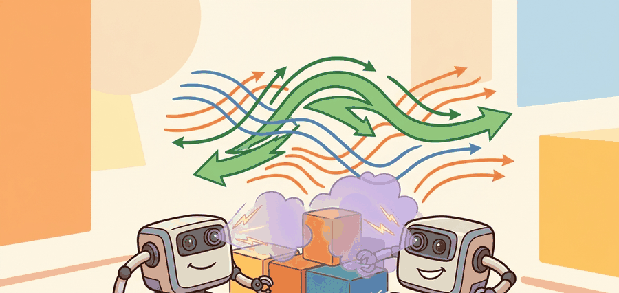
Figure 30.4.1 sketches this loop end to end: sensor measurements build a local costmap, the planner scores candidate commands against it, and the winning command leaves a trace a reviewer can later replay.

Concretely: that 0.3 second budget is several DWA control cycles at Nav2's default 20 Hz (50 ms each), which is exactly why the worked example later in this section samples and scores candidate velocities on a 0.2 s timestep rather than trying to re-plan a whole path in the moment the person steps out.

Problem First

Picture a robot rolling toward a doorway at 0.5 m/s when the global map, drawn yesterday, still insists the path is clear: in the next 50 ms it has to commit to one velocity command, and no redrawing of the route can save it from a wall that the map never knew about. A global path (the coarse route from start to goal computed over a static map) is too coarse for the next second of motion, and the local costmap (a short-range grid of obstacle cost values built fresh from the robot's current sensor data, distinct from the static global map) is what the planner actually scores commands against. The robot still has to choose velocities that avoid nearby obstacles, respect acceleration limits, and remain trackable by its controller.

The Dynamic Window Approach (Fox, Burgard, and Thrun's 1997 method, now shipped as the Nav2 DWB controller) samples feasible velocity commands and scores their short rollouts on a differential-drive base like a TurtleBot3. Potential fields, the steering law Khatib introduced for manipulator obstacle avoidance at Stanford in 1986, define attractive and repulsive forces but stall in the symmetric local minima of a doorway. Deployed stacks like ROS 2 Nav2 and Boston Dynamics Spot's autowalk combine costmap scoring, trajectory rollout, and controller constraints rather than relying on either method alone.

A velocity that cannot be executed safely in the next 50 ms is not a plan; it is a wish.

Formal Model

Most navigation methods can be read as constrained search or optimization:

$$ u^*=\arg\min_{u\in\mathcal U_{\mathrm{dyn}}}\alpha d_{\mathrm{goal}}+\beta c_{\mathrm{obstacle}}+\gamma e_{\mathrm{path}} $$

The objective is short-horizon progress; constraints are collision clearance, velocity, acceleration, curvature, obstacle prediction, and emergency stop authority.

Why this formulation matters physically. A real robot cannot pause mid-motion to replan; every 50 ms it commits to a command its actuators can execute. Encoding safety as a hard constraint, not a soft penalty, guarantees that no tradeoff of speed or path alignment can override collision avoidance. Hardware demands this: a collision, unlike a suboptimal path, is irreversible.

Tuning the weights

How the weights interact. The three scalars \(\alpha\), \(\beta\), \(\gamma\) are tuned relative to each other, not in isolation. Raising \(\beta\) (obstacle cost) causes the planner to accept larger path deviations to preserve clearance; raising \(\alpha\) (goal distance) pulls trajectories tighter to the global route at the cost of narrower safety margins. In practice, \(\beta\) is set first to guarantee a minimum clearance budget, then \(\alpha\) and \(\gamma\) are swept together to balance goal-seeking against path tracking.

Before reading on, guess: if you double \(\beta\) relative to \(\alpha\), does the robot become faster at reaching its goal, slower but safer, or does it stall in doorways?

How DWA and Potential Fields Actually Work

With the cost function and its weights now fixed, the remaining question is which commands the planner is even allowed to score, and that is exactly where the Dynamic Window Approach and potential fields diverge.

In the Dynamic Window Approach, the planner constrains the search to velocity pairs \((v, \omega)\) reachable within one timestep given the robot's current speed and its acceleration limits. Such constraints are called kinodynamic: they combine kinematic limits (geometry and reachable configurations) with dynamic limits (the velocities and accelerations the actuators can physically produce). Take a robot moving at \(v = 0.5\) m/s with a deceleration limit of \(0.5\) m/s\(^2\) and a 0.2 s timestep. The dynamic window restricts candidate linear speeds to \([0.4, 0.6]\) m/s. The planner simulates each candidate pair forward for a short horizon (typically 2 to 3 s, sometimes called a rollout: a short forward simulation of what would happen if a candidate command were applied) and scores it on heading alignment, obstacle clearance, and speed. That kinodynamic window typically eliminates over 90% of the velocity grid before scoring begins. The same robot can reach only about 11 out of a 100-point grid in one timestep, so the planner's real search is far smaller than it appears on paper.

The Nav2 DWB controller (the Nav2-specific reimplementation of DWA with pluggable critics) runs this loop at 20 Hz (the default controller frequency as of Nav2 Humble, 2022) on a TurtleBot, selecting whichever admissible \((v, \omega)\) pair minimizes the weighted cost. Figure 30.4.2 shows this pruning step directly: the small blue box marks the dynamic window inside the full velocity grid, with green dots for commands that survive collision checking and red for those that do not.

Potential fields take a different approach. The goal exerts an attractive force proportional to distance, and each obstacle exerts a repulsive force that falls off with the square of clearance. The robot then follows the gradient of the combined field. The method is fast and memoryless, but a narrow corridor breaks it. When two repulsive walls sit symmetrically, their forces cancel and the robot stalls. This is the symmetric-repulsion deadlock. In a 0.8 m corridor with walls at equal distance, a pure potential-field robot stalls 100% of the time. DWA's velocity sampling escapes the same corridor in under 0.5 s, because it treats the passage as a feasibility constraint rather than a force balance. This local minimum problem is the central reason potential fields are rarely used alone in deployed systems.

Worked Diagnostic

Code Fragment 1 isolates local-planner scoring: candidate command, obstacle clearance, progress term, and dynamic feasibility. The point is to make command rejection inspectable.

# Score three local velocity commands.
# The selected command balances goal progress and obstacle clearance.
candidates = [
    {"v": 0.6, "goal": 2.0, "clearance": 0.20},
    {"v": 0.4, "goal": 2.4, "clearance": 0.55},
    {"v": 0.2, "goal": 3.0, "clearance": 0.80},
]
scores = []
for c in candidates:
    score = c["goal"] + 1.5 / c["clearance"] - 0.3 * c["v"]
    scores.append((round(score, 2), c["v"]))
print(scores)
print(f"command_v={min(scores)[1]}")

Expected output interpretation. The smallest score belongs to the slowest command because clearance dominates goal progress in this local decision. That is the intended interpretation of the output: when hazards are near, the local planner should sacrifice speed first, rather than preserving nominal throughput at the cost of safety margin.

That same clearance-first scoring, small enough to inspect in a dozen lines here, is precisely the logic that production navigation stacks scale up to thousands of robots on a live floor.

Tool Workflow

Keep the small DWA or potential-field fragment as a test for cost terms and constraints. Use Nav2 controllers and behavior trees (the modular, tree-structured control logic that sequences navigation tasks like planning, recovery, and retry without a monolithic state machine) when deploying on a full robot.