"Motion cues matter when they change what the robot should do before the next frame arrives."
A Patient Embodied AI Agent
This section assumes familiarity with the brightness constancy model introduced in section 27.1 and with the sensor timing concepts from section 8.7. The motion-cue pipeline developed here feeds directly into the affordance reasoning of section 27.5 and the collision-avoidance planner of section 30.4. Systematic failure testing of optical flow under camera shake and rolling shutter is covered in section 27.7.
A drone flying down a corridor at 8 m/s has roughly 80 milliseconds before a door frame fills its field of view. No semantic detector identifies "door frame" in that window. But the expanding optical flow pattern, that radial bloom of pixel velocities, does. Optical flow is the fastest control-relevant signal a visual system can produce, and modern embodied AI finally has the compute to run it dense, in real time, on-board. This section develops a flow pipeline, decomposes it into ego-motion and object-motion components, and wires the result to a reactive controller that brakes before slower perception ever wakes up.
Problem First: Why This Representation Exists
Optical flow is not just a visualization of motion. A flow field that never changes a control command is a screensaver, not a perception system. In embodied systems it is a short-horizon warning signal whose value depends on frame timing, ego-motion compensation, and action latency.
The contract here maps frame pairs to action timing: flow field, camera motion estimate, dynamic-object hypothesis, uncertainty, update rate, and the reactive controller that consumes it.
Flow becomes embodied knowledge when it changes braking, pursuit, gaze, manipulation timing, or collision avoidance before a slower semantic pipeline can respond.
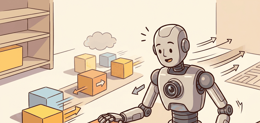
Figure 27.4.1 should be read as a motion-cue contract: flow field, ego-motion compensation, object motion hypothesis, latency, and controller consumer determine whether motion changes the next command.
Mathematical Core
Having framed flow as a timing contract, the next step is the equation that turns two frames into a velocity field. Classical optical flow starts with brightness constancy and a small-motion approximation.
\(I_x u + I_y v + I_t = 0,\quad \tau \approx \frac{\theta}{\dot\theta}\)
The first equation says that image intensity should stay constant as a point moves. The time-to-contact approximation uses visual expansion: when an object's angular size grows quickly, the robot may need to brake even before full 3D reconstruction is available.
Why this matters for embodied AI: Brightness constancy breaks whenever a robot arm casts a moving shadow, a warehouse light flickers, or fast joint motion blurs the frame. On a physical robot those violations are the norm, not the exception. A flow estimate computed under violated brightness constancy can report phantom obstacles or miss real ones. It then brakes in a clear corridor or fails to stop before a real pedestrian. So treat brightness constancy as a calibration target. Characterize the robot's operating environment for lighting stability, and make the flow pipeline carry a per-pixel confidence that drops when the assumption likely fails.
Deriving the constraint
How the equation is derived: Take the image intensity \(I(x, y, t)\) at a pixel. If that pixel moves by \((dx, dy)\) in time \(dt\), brightness constancy asserts \(I(x+dx, y+dy, t+dt) = I(x, y, t)\). A first-order Taylor expansion of the left side gives \(I + I_x dx + I_y dy + I_t dt = I\). This simplifies to \(I_x u + I_y v + I_t = 0\), where \(u = dx/dt\) and \(v = dy/dt\) are the pixel velocities we want. This single equation has two unknowns, so each pixel is underdetermined. A smoothness constraint resolves the aperture problem: Lucas-Kanade assumes constant flow in a local window, and Horn-Schunck adds a global regularizer (an extra penalty term that discourages the flow field from changing abruptly between neighboring pixels, trading some accuracy at true motion boundaries for a smoother, more stable field overall). Each choice trades noise tolerance against sensitivity to motion discontinuities at object boundaries.
The aperture problem is like watching a striped scarf slide past a keyhole: through the hole you can see the stripes moving, but you cannot tell whether the scarf is moving sideways, diagonally, or even along the stripe direction, because all of those motions look identical through that tiny opening. Only by widening your view to a patch of fabric that includes a corner, a button, or a contrasting edge can you pin down the true direction of travel. Lucas-Kanade does exactly that: it pools evidence from a small neighbourhood of pixels so that nearby features with different orientations vote together and resolve the ambiguity that any single pixel leaves open.
Checkpoint
So far: brightness constancy gives one equation per pixel with two unknowns (the aperture problem), and Lucas-Kanade or Horn-Schunck resolve that ambiguity by pooling evidence from neighboring pixels; the payoff is the flow-to-action recipe below, which turns that pooled flow field into a concrete slow, stop, or replan command.
- Estimate sparse or dense flow between consecutive frames.
- Subtract expected ego-motion flow when camera motion is known.
- Cluster residual flow into moving object hypotheses.
- Convert expansion, bearing change, or residual speed into a controller-level slow, stop, or replan signal.
Worked Decomposition: separating ego-motion from object motion
Step 2 of the recipe ("subtract expected ego-motion flow") is the part this section promises but has not yet shown numerically. Suppose the camera is panning at an angular rate of 0.20 rad/s and a pixel sits 300 pixels from the image center with a focal length of 500 pixels. The expected ego-motion flow at that pixel is approximately \(\dot\theta \times f = 0.20 \times 500 = 100\) px/s directed opposite the pan. If the observed flow at that pixel is 130 px/s in the same direction, the residual after subtraction is \(130 - 100 = 30\) px/s: a small but genuine object-motion signal, not the full 130 px/s a naive detector would have flagged. This is exactly the arithmetic behind the "Separate ego or object" stage in Figure 27.4.1 and the phantom-obstacle failure discussed below: skip the subtraction and the controller reacts to 130 px/s of pure camera rotation.
The table below contrasts three common flow strategies so you can pick one against your compute budget and the control risk you can tolerate.
| Design Choice | Use When | Control Risk |
|---|---|---|
| Sparse feature flow | Visual odometry and low-compute tracking | Fails on textureless surfaces and repetitive patterns. |
| Dense learned flow | Scene motion and manipulation video | Can be expensive and may hallucinate in occlusion. |
| Residual flow | Moving obstacle detection | Bad ego-motion compensation can create false obstacles. |
Worked Miniature
Code Fragment 27.4.1 uses bounding-box size over time to estimate a simple time-to-contact cue. It is not a replacement for full flow, but it teaches the control signal hidden inside motion.
# Estimate time-to-contact from visual expansion.
# A smaller tau means the controller should slow or stop sooner.
import numpy as np

box_width_px = np.array([42.0, 48.0, 56.0, 67.0])
dt_s = 0.10
growth_rate = (box_width_px[-1] - box_width_px[-2]) / dt_s
tau_s = box_width_px[-1] / growth_rate
command = "slow" if tau_s < 1.0 else "continue"
print(round(float(tau_s), 2))
print(command)tau_s from four bounding-box width samples (42.0 to 67.0 px at 0.10 s intervals) and emits a `slow` command once the growth rate pushes tau_s below the 1.0 s threshold.Step-Through: time-to-contact from box expansion
Trace the recipe with the four widths in Code Fragment 27.4.1, sampled at 0.10 s intervals: 42.0, 48.0, 56.0, 67.0 px. The growth rate uses the last two samples: \((67.0 - 56.0) / 0.10 = 11.0 / 0.10 = 110.0\) px/s. The current size is 67.0 px, so \(\tau = 67.0 / 110.0 = 0.609\) s, which rounds to 0.61 s. Because 0.61 is below the 1.0 s threshold, the command flips to slow. Now watch the cue sharpen frame by frame: between samples 1 and 2 the rate was \((48-42)/0.10 = 60\) px/s giving \(\tau = 48/60 = 0.80\) s; between samples 2 and 3 it was \((56-48)/0.10 = 80\) px/s giving \(\tau = 56/80 = 0.70\) s. The shrinking 0.80 to 0.70 to 0.61 s sequence is the expanding-flow signature: the object is not just close, it is closing, and the controller sees that one sample before any depth map confirms it.
OpenCV provides Lucas-Kanade and Farneback flow, while modern PyTorch models provide learned dense flow. Those tools reduce implementation work, but the robot still needs ego-motion compensation, latency checks, and a controller policy for residual motion.
RAFT (Recurrent All-Pairs Field Transforms, Teed and Deng 2020) builds a 4D correlation volume (a lookup table of how well every pixel in frame t matches every candidate pixel in frame t+1, across all four spatial dimensions) over every pixel pair across two frames, then refines the flow field with a recurrent unit (a small neural network applied repeatedly, each pass sharpening the previous flow estimate rather than computing it from scratch). It reaches an average end-point error below 1.5 pixels on Sintel, a synthetic-animation benchmark dataset widely used to score optical-flow accuracy against known ground truth, but runs at only about 10 fps on a 720p frame with a 2020-era mid-range GPU (typically 20-30 fps on 2024 hardware). At that 100 ms latency, a robot moving at 1 m/s travels 10 cm blind before the estimate lands. The bounding-box expansion of Code Fragment 27.4.1 returns a hint in under 2 ms on the same GPU: 50 times faster for roughly half the accuracy. That asymmetry is why bounding-box time-to-contact earns a parallel low-latency channel alongside learned flow, and why the closed-loop controller must budget end-to-end sensor-to-actuator latency.
When running RAFT (or any learned dense-flow model) in a robotics pipeline, consider passing iters=12 rather than the default iters=32 during online inference: in practice, 12 recurrent update steps typically recovers more than 95% of full-iteration accuracy on robot scenes similar to those reported in the RAFT ablations, while cutting GPU time roughly in half, though the exact tradeoff depends on scene texture and motion magnitude. Also set mixed_precision=True at model construction; without it RAFT allocates a full float32 correlation volume that can exceed 2 GB on 720p frames, which on devices with less than 4 GB VRAM can silently fall back to CPU, making latency appear acceptable in benchmarks but catastrophic on the actual hardware.
A common assumption is that optical flow directly measures how fast objects are moving in the physical world. This is wrong: flow measures pixel displacement in the 2D image plane, not 3D velocity. A pedestrian one meter away and a pedestrian ten meters away moving at the same physical speed produce very different flow magnitudes, and a perfectly stationary wall produces large flow when the robot turns. In embodied AI the correct mental model is that flow is a 2D image-plane signal that must be combined with depth estimates, ego-motion data, and camera calibration before it can drive any metrically accurate control decision.
Do not treat every flow vector as object motion. A turning camera creates global flow, so the system must subtract expected ego-motion before labeling a pedestrian, arm, or drone as moving.
Ego-motion compensation can fail silently. The standard approach projects Inertial Measurement Unit (IMU) angular velocity into expected pixel displacement and subtracts it from the observed flow field. This works only when the IMU and camera are time-synchronized to within a few milliseconds and the intrinsic calibration is fresh. On a wheeled robot hitting a bump, IMU integration typically drifts for on the order of 50 to 100 ms, producing a residual flow pattern that can look like a moving obstacle at the robot's heading. The system may then issue a false slow or stop command with no visible error signal, because the residual is non-zero and spatially coherent. It is like a car's windshield briefly fogging after a pothole: the road ahead is clear, but the driver sees an obstacle where there is only smeared glass. Always log raw flow, expected ego-flow, and residual separately so this failure is reproducible offline.
An indoor delivery robot can use residual flow to slow for a person stepping from behind a shelf, combining the motion cue with local obstacle avoidance for a safe stop command. The action policy should log whether the stop came from obstacle geometry, optical expansion, or a conservative fallback.
Real-World Application: drone obstacle avoidance
Skydio drones run dense optical flow as part of their onboard visual navigation stack, fusing flow-derived motion with depth from six fisheye cameras to fly through forests and around moving people without a prior map. The expanding-flow time-to-contact cue is exactly what lets the aircraft brake or veer in the tens-of-milliseconds window before a branch or person fills the frame, well faster than any semantic detector could label the obstacle.
The perception result must answer what action changed, what uncertainty changed, and what log would reproduce the decision. Otherwise the output is still visualization, not embodied evidence.
Debugging And Evaluation
Because the value of a flow pipeline is defined entirely by the actions it changes, the only honest way to test it is to log those actions next to the motion evidence that triggered them. Evaluate motion cues with time-aligned logs: record frame pair, optical flow summary, ego-motion correction, predicted moving obstacle, chosen action, latency, and near-miss label.
Perturb frame rate, motion blur, rolling shutter, camera shake, and independently moving objects, then check whether the action changes because of motion rather than texture. Section 27.7 catalogs how perception failures become action failures when these perturbations are not tested systematically.
Long-horizon point tracking as a manipulation primitive. CoTracker3 (Karaev et al., 2024), a model that follows individual chosen points across an entire video rather than computing flow only between adjacent frame pairs, tracks arbitrary point clouds across long video sequences with sub-pixel drift, enabling robots to maintain contact-point identity through occlusion across 30-plus frames. Physical robotics groups at CMU and ETH Zurich are exploring how persistent point tracks replace object-level bounding boxes as the control signal for dexterous in-hand manipulation, where the object pose changes continuously and a box centroid loses meaning.
Flow-guided world models for policy learning. UniSim (Yang et al., 2024, Google DeepMind), a learned simulator that predicts what a scene will look like after a candidate action without executing that action on real hardware, and related work use predicted optical flow as an intermediate representation inside learned world models, letting a policy simulate the visual consequence of an action before committing to it. The key finding is that a model conditioned on flow residuals generalises to novel object shapes better than one conditioned on raw RGB, because flow encodes physically plausible motion rather than appearance. Several 2025 follow-ons (including work from Freiburg's Robot Learning Lab) apply this idea to contact-rich assembly tasks where appearance varies across lighting conditions but flow patterns remain stable.
Event-camera optical flow at microsecond latency. Traditional frame-based flow has an irreducible latency floor set by the inter-frame interval. Event cameras (Dynamic Vision Sensors) fire asynchronous spikes at each pixel the moment brightness changes, enabling flow estimates with sub-millisecond latency. TUM's DSEC benchmark, a stereo driving-scene dataset pairing event-camera and frame-camera recordings for evaluating flow under difficult lighting (Gehrig et al., 2021, updated splits 2024), and the associated E-RAFT architecture, a version of RAFT adapted to consume asynchronous event streams instead of paired frames, show that event-based flow can track fast drone manoeuvres at over 200 fps equivalent with 6-10x lower power than a frame camera pipeline at the same temporal resolution, making it a strong candidate for the latency-critical reactive controller slot described in this section.
Open problem for PhD research. None of the three directions above solves uncertainty-aware flow under simultaneous ego-motion and independently moving objects on power-constrained hardware. Specifically: given a mobile manipulator arm that is itself moving while a human hand enters the workspace, how should a system decompose the total flow into arm self-motion (predictable via forward kinematics), camera ego-motion (predictable via IMU), and residual intrusion flow (the signal of interest), and how should it propagate a per-pixel uncertainty through that decomposition so that the reactive controller knows when to trust a slow command? Current systems handle each component separately; a joint probabilistic formulation that remains within a 10 ms latency budget on a 30 W edge GPU does not yet exist.
Project Ideas
Beginner (weekend): Build a time-to-contact alerter using OpenCV's Lucas-Kanade sparse flow on a webcam feed: compute bounding-box expansion for a tracked object and publish a "slow" signal when tau falls below one second. The key challenge is filtering spurious expansion spikes caused by lighting changes without adding enough lag to defeat the low-latency purpose of the signal.
Intermediate (1-2 weeks): Implement an ego-motion-compensated moving-obstacle detector in a Gymnasium environment rendered with PyBullet: use the simulator's known camera pose to compute expected background flow, subtract it from RAFT dense-flow output, and cluster residuals into dynamic-object hypotheses that feed a reactive stop command. The key challenge is keeping end-to-end latency inside one control cycle (33 ms at 30 Hz) when RAFT at default iteration count already costs 80-100 ms on a mid-range GPU, requiring you to tune iteration depth and resolution without destroying accuracy on the moving-obstacle case.
Advanced (3-4 weeks): Wire a flow-based collision-avoidance policy into a LeRobot manipulation stack running in Isaac Lab: the robot arm should detect when a human hand enters its workspace via residual flow and pause mid-trajectory, then resume once the residual drops below threshold. The key challenge is separating arm self-motion flow (large, predictable, ego-motion) from hand intrusion flow (smaller, unpredictable) using forward-kinematics-projected pixel velocities rather than IMU data, which is absent for a stationary arm.
Section 27.5 extends motion-driven avoidance into intentional contact: once the robot knows what is moving and where, affordances let it decide which regions it can actually grasp, push, or step on.
Section References
OpenCV. Optical flow tutorials. https://docs.opencv.org/4.x/d4/dee/tutorial_optical_flow.html
Documents classical sparse and dense optical-flow tools used in practical robotics prototypes.
NVIDIA. Isaac ROS Visual SLAM documentation. https://nvidia-isaac-ros.github.io/repositories_and_packages/isaac_ros_visual_slam/index.html
Shows real-time visual motion estimation in a ROS 2 robotics stack.
Can you name the representation, the consuming action, the uncertainty or freshness field, and the failure label for Optical flow and motion cues? If any one is missing, the section is not yet ready for a robot replay log.
Lab: watch ego-motion masquerade as an obstacle
Goal: see for yourself how a turning camera produces global flow that a naive detector mislabels as a moving obstacle, then confirm that ego-motion subtraction removes the phantom. Budget 20 to 30 minutes.
Tools: Python with OpenCV (pip install opencv-python) and a webcam, or any short clip with both pure camera pans and a genuinely moving object. Use cv2.calcOpticalFlowFarneback for a dense field.
Steps and what to vary: (1) Hold the camera still and wave one hand across the frame; visualize flow magnitude as a heatmap and note the localized bright blob. (2) Keep the scene static and pan the camera left to right; observe that the entire frame now lights up. (3) Estimate the dominant global flow (the median flow vector over the whole field) and subtract it from every pixel, then re-render the residual heatmap.
What to observe: in step 2 the unsubtracted field flags the whole wall as moving, the classic phantom obstacle; after subtraction in step 3 the static scene goes dark while a truly moving hand still survives as residual. Vary pan speed and lighting to find where median subtraction breaks down (fast rotation, rolling shutter, low texture), which is the exact failure surface section 27.7 tests systematically.
Optical flow is not just pretty arrows; it is a low-latency motion signal that must be separated into ego-motion, object motion, and control response.
Design a residual-flow test for a mobile robot turning in place while a person walks across the scene. What flow should be subtracted, and what residual should trigger slowing?